Building circadian ontogenetic metabolomics atlas (COMA)

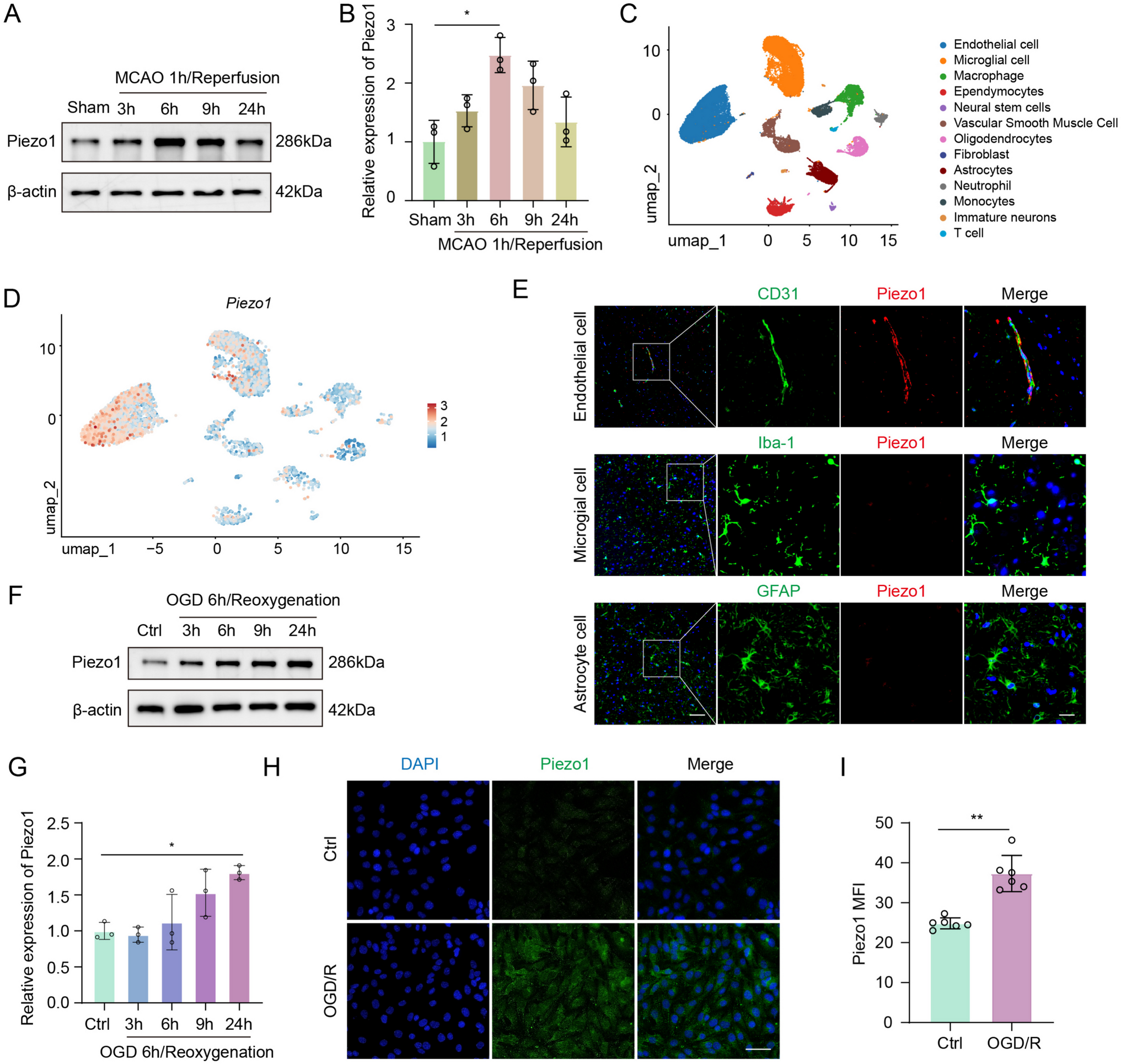
We have studied the development of the circadian metabolome of rat brain, specifically in the SCN and mPFC, as well as in peripheral tissues such as the liver and plasma. This study spans five developmental stages, including embryonic E19 and postnatal stages P2, P10, P20, and P28 (see Fig. 1). Fecal samples were collected at all postnatal stages. For postnatal stages P20 and P28, additional tissues were collected, including the kidney, heart, lungs, spleen, pancreas, small intestine (jejunum), stomach, gastrocnemius skeletal muscle, isWAT, dlWAT, and iBAT. Sampling was conducted at Zeitgeber times 0, 4, 8, 12, 16, 20, and 24 h for all developmental stages. Following a well-established approach, clock gene analysis was also performed for SCN, liver, pancreas, and dlWAT.

Fig. 1

Graphic illustration of the workflow toward building circadian ontogenetic metabolomics atlas of rat plasma, tissues, and feces

As the construction of comprehensive mass spectrometry-based metabolomics and lipidomics atlases is an emerging field [44], we provide detailed information below and in the experimental section on sample preparation, instrumental platforms, data processing and curation, as well as quality control.

We analyzed 1610 study samples using untargeted LC–MS-based metabolomics platforms, accompanied by method blanks and quality control samples. To reduce extract complexity, we employed an “all-in-one” extraction approach (LIMeX) with methanol, methyl tert-butyl ether, and water [46, 47], resulting in two phases: the upper one containing nonpolar metabolites (complex lipids) and the bottom one mostly consisting of polar metabolites. The optimal plasma volume, tissue amount for extraction, collected aliquots, resuspension solvent volumes, and injection volumes were determined during a pilot study. The final injection volumes were confirmed using quality control samples before analyzing all study samples.

Each of these fractions underwent analysis under different separation conditions: HILIC for highly polar metabolites such as amino acids, biogenic amines, sugars, nucleotides, acylcarnitines, and sugar phosphates; RPLC for medium polar metabolites; and RPLC analysis of complex lipids. The optimal conditions of each LC–MS platform were based on our previously published methods [47], incorporating a high-throughput approach with each sample analyzed in less than 5 min [46].

LC–MS/MS raw data were processed using MS-DIAL software [53], including annotating polar metabolites (metabolomics workflow) and complex lipids (lipidomics workflow). All mass spectra underwent manual investigation, utilizing retention times and mass spectral information from MS1 and MS/MS libraries. To assess the precision of the overall analytical method, a superior quality control (SQC) sample was prepared by pooling QC samples from each matrix to reflect an aggregated metabolite composition. This SQC sample was aliquoted and repeatedly injected after every set of 35 samples (Fig. S1) and used to correct longitudinal signal drifts using locally estimated scatterplot smoothing (LOESS).

Overall analytical precision was evaluated through PCA of the total variance. As shown in the PCA score plot (Fig. S2), the tight clustering of SQC injections indicates minimal residual technical variability. In contrast, metabolomic and lipidomic profiles from different rat samples were more dispersed, with the first two principal components explaining over 42% of the total biological variance. Analysis of the SQC samples revealed that 84% of all annotated metabolites had excellent reproducibility, with relative standard deviations (RSD) below 10%. Furthermore, 99.2% of metabolites showed RSD values below 20%, underscoring the high quality and consistency of the dataset (Table S1). In total, 851 distinct metabolites were annotated and passed the quality control criteria (see Supplementary materials and methods). Coloring the PCA plots by matrices revealed clear biological differences among sample types. Fig. S3 shows samples from the SCN, mPFC, plasma, and feces formed distinct clusters, indicating pronounced metabolic differences in these compartments. In contrast, other tissue samples exhibited greater overlap, reflecting more subtle metabolic variation.

The annotated metabolites were used for subsequent statistical analyses, including JTK_CYCLE, a nonparametric algorithm for detecting rhythmic components in large datasets [51], and the recently introduced dryR algorithm, which assesses differential rhythmicity in time series data [52]. In addition, the metabolites were also included in multivariate analyses such as PCA and PLS-DA to provide an overview of the dataset [54].

As anticipated, complex lipids constituted the majority of reported metabolites (71%) due to their high endogenous content in various biological matrices. Main lipid classes included (lyso-)phosphatidylcholines (LPC, PC), (lyso-)phosphatidylethanolamines (LPE, PE), triacylglycerols (TG), free fatty acids (FA), acylcarnitines (CAR), phosphatidylserines (PS), phosphatidylinositols (PI), phosphatidylglycerols (PG), sphingomyelins (SM), ceramides (Cer), and diacylglycerols (DG). Organic acids, amino acids, modified amino acids, peptides, hydroxy acids, organic oxygen compounds, organoheterocyclic compounds, organic nitrogen compounds, nucleosides, nucleotides, and others were the main components of the polar metabolome.

Furthermore, the RT qPCR method [45, 48] was employed to detect mRNA levels of clock genes in the liver (Per1, Per2, Rev-Erbα, Cry1, Bmal1, Clock), SCN (Per2, Rev-Erbα, Bmal1, Dbp, E4bp4), pancreas, and dlWAT (Per2, Rev-Erbα) for further investigation of the rhythmicity during ontogenesis.

Web application

The dataset for this study comprises 1610 samples, each containing hundreds of annotated metabolites, including polar metabolites and complex lipids. Clock gene data are also available for four matrices: liver, SCN, pancreas, and dlWAT. Consequently, we developed the Circadian Ontogenetic Metabolomics Atlas (COMA), a web-based application for facilitating data visualization and interpretation (https://coma.metabolomics.fgu.cas.cz).

The atlas is structured into five main sections (Fig. 2A), offering circadian profiles and outcomes of JTK_CYCLE and dryR algorithms for polar metabolites and complex lipids in matrices, a general overview of detected metabolites in matrices for each developmental stage, clustering of circadian metabolites in matrices, multivariate data analysis of metabolites in matrices irrespective of time points, and study design.

Fig. 2

Circadian Ontogenetic Metabolomics Atlas website. (A) The initial web page of the Circadian Ontogenetic Metabolomics Atlas; (B) example of data visualization of the amino acid citrulline in plasma (PLS) and the liver (LIV) in the “Metabolites” section using the original dataset and JTK_CYCLE algorithm. Oscillating metabolites (p<0.05, Bonferroni-adjusted for multiple testing, ADJ.P) are colored by default, while non-oscillating metabolites are gray

The “Metabolites” section overviews all polar metabolites and complex lipids. Users can search for a specific metabolite by name, molecular formula, and InChIKey. Additional search options for complex lipids include the number of carbons and double bonds. The “Metabolomics” section is further divided into “Complex lipids” and “Polar metabolites.” Profiles and outcomes of the JTK_CYCLE and dryR algorithms are displayed when selecting particular metabolites. Data are visualized for each developmental stage (E19, P2, P10, P20, and P28), along with the collected matrix and the calculated adjusted p-value (see an example of the amino acid citrulline) in Fig. 2-B. Oscillating metabolites (p < 0.05) are colored by default, while non-oscillating metabolites are gray. Users can adjust the p-value threshold according to their preferences. Results are available to the entire dataset without outlier detection (marked as the “Original” dataset) and after removing outliers based on the median value and the absolute deviation from the median, using upper and lower limits determined 4 times the median absolute deviation (marked as the “Outlier-free” dataset). Changes take effect after clicking the “Refresh plot” button, enabling users to compare the outcomes of both data pretreatment approaches.

The “Overview” section provides a general overview of the composition of the analyzed matrices for each developmental stage. A sunburst graph visualizes hierarchical data in concentric circles, displaying the total number of unique annotated metabolites for each matrix and developmental stage, sorted into polar metabolites, complex lipids, and their respective classes. It also presents the total number of circadian metabolites identified using the JTK_CYCLE or dryR algorithms with a significance level of p < 0.05. Datasets without and with outlier detection were used, and metabolites with p-values above the threshold (0.05) are depicted in gray.

The “Clustering” section introduces categories for each matrix and developmental stage, combining JTK_CYCLE (p < 0.05) [51] and fuzzy c-means clustering [40, 55]. Six key categories indicate metabolite clusters with specific temporal dynamics based on the initial evaluation of each developmental stage and matrix, and considering typical clusters reported in the literature [40, 56]. The line width and opacity on each graph indicate the number of metabolites.

The “Explorer” section encompasses a statistical analysis of analyzed matrices, irrespective of Zeitgeber times. Matrices are categorized into digestive (liver, pancreas, stomach, small intestine), excretory (kidney, feces), respiratory (lungs), endocrine (spleen, isWAT, dlWAT, iBAT), muscular (gastrocnemius skeletal muscle), cardiovascular (plasma, heart), and nervous (SCN, mPFC) systems. Results of multivariate data analysis are presented using unsupervised PCA to visualize the first two principal components through scores and loadings plots. Supervised PLS-DA is displayed with the first two components in scores and loadings plot formats, featuring a color-based gradient indicating VIP scores for all metabolites. In both PCA and PLS-DA, samples in score plots are color-coded based on the developmental stage. A sunburst graph offers a comprehensive overview of annotated metabolites in a specific matrix. Box plots are also presented for each metabolite sorted by VIP, and clicking on another metabolite updates the corresponding box plot.

The “Study design” section summarizes experimental conditions, including details about experiments involving animals, the methodology employed, and abbreviations utilized throughout the atlas.

Clock genes are accessible using the upper panel, and the data are visualized similarly to that of metabolites. This panel also includes a download section where users can download the whole data set, including metadata.

Exploring the circadian ontogenetic metabolomics atlas

In the following examples, we provide a snapshot of the results of the Circadian Ontogenetic Metabolomics Atlas, including the investigation of circadian metabolites in each matrix and developmental stage, the clustering of metabolites, and finally, general exploration using multivariate data analysis.

The results from applying the JTK_CYCLE and dryR algorithms to identify and characterize cycling metabolites are shown in Fig. 3. The figure provides an overview of the percentage of circadian metabolites, defined as those with adjusted p-values (< 0.05; ADJ.P for JTK_CYCLE and padj for dryR) and a period (PER) of 24 h. Across matrices and developmental stages, the average percentage of oscillating metabolites was approximately 24% with JTK_CYCLE and 12% with dryR. Stomach tissue, SCN, and mPFC were identified with the lowest number of circadian metabolites, while dlWAT, isWAT, liver, and plasma had the highest number of circadian metabolites.

Fig. 3

Overview of the total number and percentage of circadian metabolites by matrix and developmental stage. The original dataset (without outlier analysis) was processed using (A) JTK_CYCLE, considering metabolites with Bonferroni-adjusted p<0.05 (ADJ.P) as statistically significant, and (B) dryR, considering metabolites with Benjamini–Hochberg-adjusted p<0.05 (padj) as statistically significant

An example of the clustering of metabolites is provided in Fig. 4 on plasma samples for all five developmental stages, illustrating commonalities in their temporal dynamics. These categories of the clusters can be characterized as follows:

(A)

Metabolites with a gradual increase during the daytime inactive phase, reaching a maximum of around 4–8 h, followed by a decrease with a minimum at 16–20 h;

(B)

Metabolites with a gradual decrease during the daytime inactive phase, reaching a minimum of around 4–8 h, followed by an increase with a maximum at 16–20 h;

(C)

Metabolites exhibiting a gradual increase during the daytime inactive phase and a rapid decrease when feeding starts at night;

(D)

Metabolites rapidly decreasing at the onset of the inactive phase, rising upon feeding until plateauing in the middle of the night;

(E)

Metabolites exhibiting a gradual increase during the daytime inactive phase and a rapid decrease when feeding starts at night;

(F)

Metabolites with a shallower decline during the inactive phase, a temporary decrease at the onset of feeding, followed by an increase 2 h after feeding begins.

Fig. 4

Cluster analysis of plasma samples by developmental stage. Six clustering categories are shown. Only polar metabolites and complex lipids with significant circadian oscillation (JTK_CYCLE, ADJ.P<0.05) were included in the analysis

For the E19 developmental stage, cluster A contained the highest number of metabolites (32%) within the clusters, whereas for P2 and P10, metabolites in cluster F dominated (45% and 65%, respectively). In the late developmental stage P20, cluster B exhibited the highest number of metabolites (42%), while metabolites in cluster A dominated the developmental stage P28 (40%). These data suggest that metabolite profiles undergo significant changes during ontogenesis.

Since the lipidome constituted the largest proportion of reported metabolites, we also implemented downloaded lists of lipids formatted for a recently introduced web-based tool called Lipid Over-Representation Analysis (LORA) [57]. LORA determines whether a priori-defined set of lipids is more present (over-represented) in a subset of lipids than would be expected by chance. A list of query lipids can be downloaded from the “Cluster” section for each matrix and developmental stage. Additionally, the entire reference lipidome can be obtained from the “Download” section (lipidome_universe.csv) and uploaded to the LORA tool at https://lora.metabolomics.fgu.cas.cz. Fig. S4 illustrates an example of plasma at the P28 developmental stage for cluster A, revealing 127 statistically significant metabolites, most of which (n = 120) are complex lipids. The UpSet plot helps identify the main structural features of enriched lipids and highlights important lipids in a graphical representation, particularly TGs containing 10:0, 12:0, and 14:0 fatty acyl chains. Using the cardinality bar plot, the cluster with the highest term intersection size (n = 18) contained TGs with a 10:0 fatty acyl chain. The second cluster contained 14 lipid species with TGs containing a 12:0 fatty acyl chain.

Furthermore, the atlas can also be used for a more general audience using the “Explorer” function. Using PLS-DA and VIP scores, it became apparent that distinct metabolites were characteristic of the analyzed matrices. For instance, in plasma, inosine (a nucleoside) dominated during the fetal E19 stage, continuously declining in postnatal stages. In the liver, glycocholic acid (a bile acid) was completely absent during fetal and early postnatal P2 and P10 stages and dominated in the P20 and P28 stages (Fig. 5A, B). In the SCN, the lipid PI 32:0 was also absent during the fetal and early postnatal P2 stage and increased over the P10, P20, and P28 stages (Fig. 5C). Similarly, HexCer 42:1;O2 was detected at higher levels in mPFC during postnatal P20/P28 stages (Fig. 5D). In feces, the vitamin riboflavin dominated during the early postnatal P2/P10 stages and was almost absent in the P20/P28 stages (Fig. 5E). These examples also show that the metabolome undergoes dramatic changes from the fetal to late postnatal developmental stages. For the rest of the matrices collected at the P20 and P28 postnatal stages, differences were observed in a way that a few metabolites occurred only in one developmental stage or differed in their intensities for most of them. These data also underscore the critical role of sampling time in metabolomics analyses, as the intensity of specific metabolites can vary significantly based on the time of collection and developmental stage. Metabolites are influenced by circadian rhythms, which govern biological processes and fluctuate throughout the day and night. This timing-dependent variation can impact the detection and quantification of metabolites, potentially leading to biased or inaccurate interpretations if sampling is inconsistent. Using animals within the same developmental stage, or “age-matched” subjects, alongside standardized sampling times, is essential to minimize variability and improve sample comparability.

Fig. 5

Box plots for the most discriminating metabolites in (A) plasma, (B) liver, (C) SCN, (D) mPFC, and (E) feces at different developmental stages based on PLS-DA and VIP

Users can also explore the analysis of clock genes. For instance, Bmal1, Per2, Nr1d1, and Dbp, in the SCN, revealed shallow rhythms at E19, followed by initiation at P2. Rhythms increased at P10, and high amplitude was observed at the P20 and P28 developmental stages (Fig. S5), as observed before in fetal E20 and early postnatal P1, P2 [58], and P10 [59] developmental stages, as well as in adult rats [11].

Potential for the discovery of novel metabolites

Hundreds of unique metabolites can usually be annotated while combining multiple platforms during untargeted metabolomics and lipidomics analyses. However, many more signals can be detected, characterized by retention time and m/z (i.e., molecular features) [60]. The raw LC–MS instrumental files provided with this atlas can be reprocessed, including updated MS/MS libraries, to increase the annotation rate further, or researchers can focus on the structural elucidation of unknown metabolites.

For example, we initially observed an unknown with a retention time of 2.2 min and m/z 188.1757 without any positive spectral match when using the combined MS/MS libraries during the HILIC platform in positive ion mode. Submitting MS1 isotopic ions and the MS/MS spectrum from MS-DIAL [53] to the MS-FINDER [61] software for structural elucidation provided over 100 possible unique structures. Since focusing on many structures would be challenging, we utilized the potential of hydrogen/deuterium exchange mass spectrometry (HDX-MS). Thus, for the HILIC–MS metabolomics platform, which uses acetonitrile/water (95:5) and water as mobile phases, both with ammonium formate and formic acid, water and mobile-phase modifiers were replaced by their deuterated forms (D2O, ammonium formate-d5, formic acid-d2). This setup permitted complete hydrogen/deuterium exchange and an additional filter from hydrogen/deuterium exchange mass spectrometry (HDX-MS) [62], reducing the number of potential candidates to one-fifth due to four labile hydrogens in the molecule as determined by a mass spectrometer. The subsequent analysis of the standard of N1-acetylspermidine confirmed the identity of this unknown based on retention time, MS1, and MS/MS spectra, including the number of exchangeable hydrogens in the parent ion and fragments (Fig. 6) when using unlabeled mobile-phase modifiers and labeled counterparts. Furthermore, N1-acetylspermidine exhibited circadian rhythmicity in different tissues at late developmental stages (P20, P28), as shown in the example of gastrocnemius skeletal muscle (Fig. 6).

Fig. 6

Structure elucidation of an unknown metabolite. (A, B) Extracted ion chromatograms (EICs) and MS/MS spectra of N1-acetylspermidine in (A) rat gastrocnemius skeletal muscle and (B) analytical standard analysis under conventional HILIC–MS with the EIC at m/z 188.1757 displayed corresponding to [M(H4)+H]+. (C, D) EICs and MS/MS spectra of N1-acetylspermidine in (C) rat gastrocnemius skeletal muscle and (D) analytical standard analysis under HILIC–HDX-MS with the EIC at m/z 193.2071 displayed corresponding to [M(D4)+D]+. (E) Circadian rhythmicity of N1-acetylspermidine in gastrocnemius skeletal muscle at the P28 developmental stage, calculated using JTK_CYCLE with a Bonferroni-adjusted p-value (ADJ.P). (F) Structure of N1-acetylspermidine