2.1 Data collection

A total of 103 pathology slides of colon cancer patients in the Third Affiliated Hospital of Heilongjiang University of Chinese Medicine from 2020 to 2023 were collected as in-house data. Four slides without grading labels were removed, and the remaining 100 cases were randomly assigned to the training and test sets. Among them, 47 cases were early colon cancer samples and 53 cases were advanced colon cancer samples. 459 colon cancer pathological sections (TCGA-COAD) were downloaded from The Cancer Genome Atlas (TCGA, https://portal.gdc.cancer.gov/) database. Three slides without grading labels were removed, 35 slides with low quality and pen and ink marks on the sections were removed, and finally 421 slides were left for subsequent analyses. Among them, there were 75 and 346 patients with early and advanced cancer, respectively. The Ethics Committee of the Third Affiliated Hospital of Heilongjiang University of Chinese Medicine approved this study. All methods were performed in accordance with the relevant guidelines and regulations of the Human Ethics Committee of the The Third Affiliated Hospital of Heilongjiang University of Chinese Medicine.

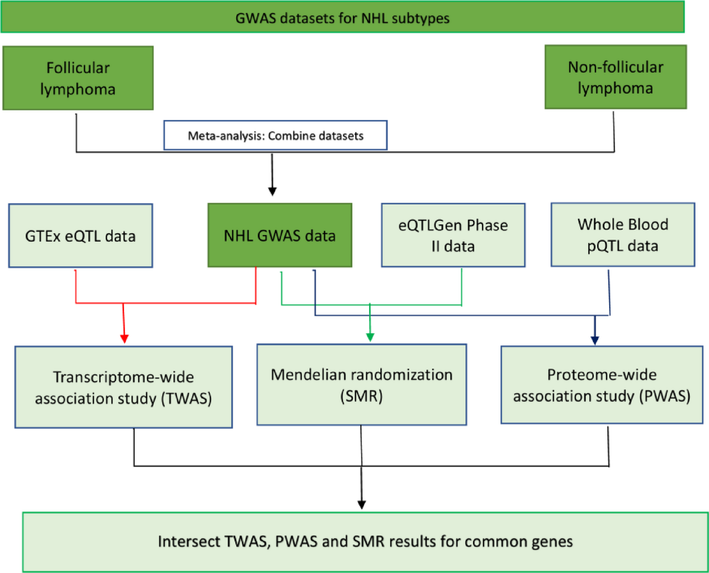
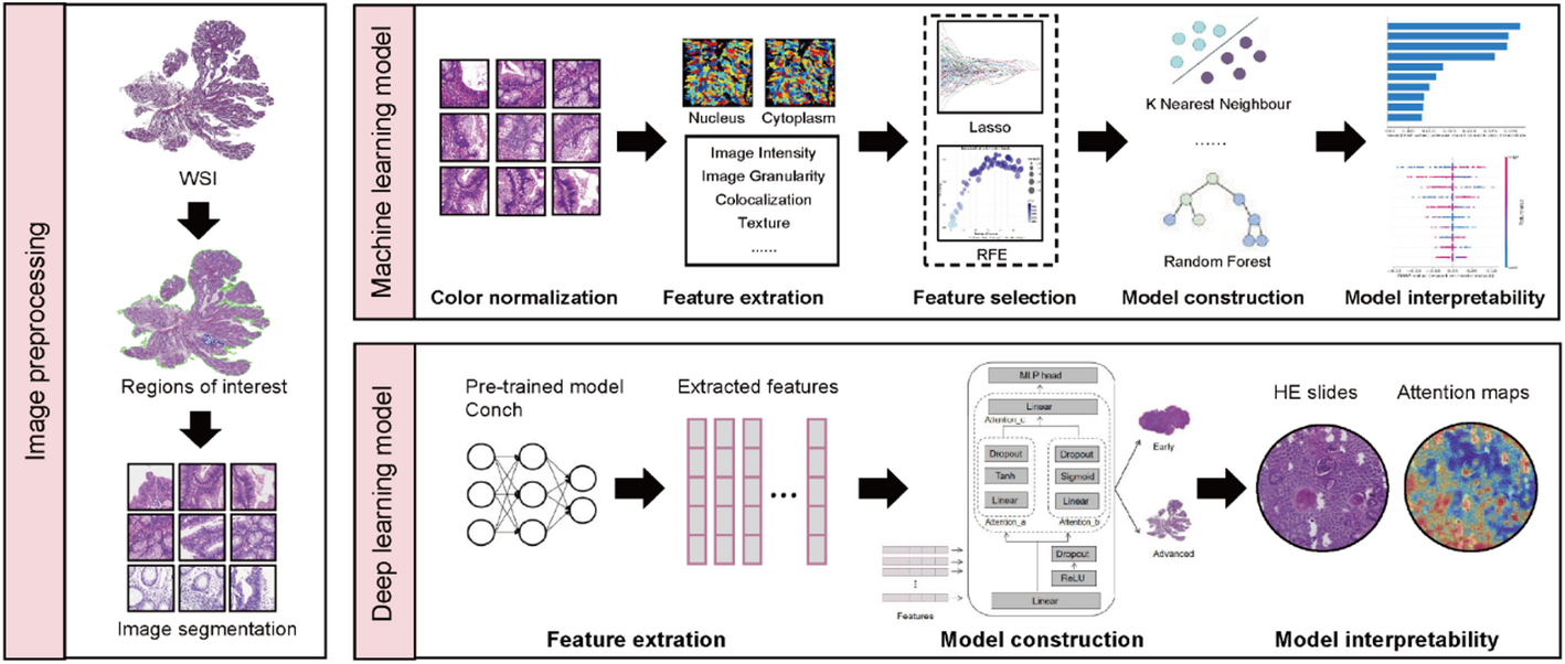
2.2 A network framework to predict tumor stage

In this study, machine learning algorithms and deep learning algorithms were used to construct colon cancer grading prediction models. Considering the origin of pathology slides, they are highly heterogeneous and contain a large number of images and high-latitude features. Therefore, this study chooses to use a variety of machine learning algorithms to train models with high accuracy and good generalization ability. Shapley Additive exPlanations (SHAP) was used to account for the importance of features. In addition, we used deep learning model ResNet50 to extract features, then added multi-layer neural network to output patch prediction results, and finally output the prediction results of the whole slice by average pooling. The important pathological features identified by the model were explained based on the attention heatmap. The flowchart for the data used in this study is shown in Fig. 1.

Fig. 1

The flowchart for the data used in this study

2.3 Machine learning training2.3.1 Data preprocessing

H&E-stained pathological sections were cut using OpenSlide-Python at a magnification of 20×, and 10 512 × 512 tiles were selected from each section as representative tiles. While the most common cause of color variation is differences in protocols and practices in histology laboratories, displayed color can also be affected by variations in capture parameters (for example, illumination and filter), image processing of the digital system itself, and display factors [17, 18]. The color of the tiles was normalized using the vahadane method to take into account the differences in the staining preparation process of the different tissues.

2.3.2 CellProfiler extracts cell features

The selected tiles were subjected to feature extraction using cellprofiler, and the H&E-stained images were firstly divided into hematoxylin-stained and eosin-stained grey-scale images using the “UnmixColors” module. Then the images were automatically segmented by “IdentifyPrimaryObjects” and “IdentifySecondaryObjects” modules to identify the nucleus and cytoplasm. Finally, the image is automatically segmented by “MeasureColocalisation”, “MeasureGranularity”, “MeasureObjectIntensity”, “MeasureObjectNeighbors”, “MeasureTexTure” to further extract quantitative image features such as object shape, size, texture, granularity, pixel intensity distribution, co-location, and so on.

2.3.3 Feature selection

Least Absolute Shrinkage and Selection Operator (LASSO) regression is a powerful feature selection method that drives the sparsification of some feature coefficients by introducing L1 regularisation to achieve feature selection [19]. Recursive Feature Elimination (RFE) finds the best subset of features by recursively constructing the model and selecting the best or worst features (based on weights), gradually eliminating unimportant features [20]. The cell features extracted by cellprofiler were firstly screened by LASSO regression analysis based on the “glmnet” R package. The results of LASSO analysed were then further filtered using the RFE algorithm in the R package “caret”. The correlation between features was visualised using the R package “corrplot”.

2.3.4 Construction of machine learning models

The selected features were used as training data, and the patient’s tumor stage was used as the training label. Multiple machine learning algorithms including XGBoost, LightGBMXT, CatBoost, LightGBMLarge, ExtraTrees, RandomForest, and KNeighbors were integrated to train the model. The tiles were stratified into 7:3 training set and test set according to clinical information, and the performance of the model was evaluated using receiver operating curves with area under curve (AUC) and confusion matrix. In addition, the TCGA-COAD data was used as an external validation set to validate the model to further illustrate the generalization ability of the model.

2.3.5 Feature importance analysis

The importance of features is explained using SHAP, a method for interpreting machine learning models based on the Shapley value theory of game theory, which provides a ranking of the relative importance of each feature by decomposing its contribution to the prediction [21]. SHAP is able to provide relative importance rankings for individual samples, individual features or combinations of features, etc., which is useful for understanding the overall behaviour of the model and its impact in a particular prediction. SHAP also provides a global model interpretation method that allows feature importance maps to be generated by calculating the average contribution of each feature over all samples. This makes SHAP one of the indispensable model interpretability tools for many machine learning tasks.

2.4 Deep learning training2.4.1 Pathological image segmentation and feature extraction

The Python-based CLAM analysis tool was used to cut the pathology slides into non-overlapping tiles with 256 × 256 pixels for feature extraction. Then, the feature vectors are extracted by feeding the cropped pixels 256 × 256 patches to the pre-trained deep network ResNet50. Finally, adaptive average space pooling was used after selecting the third residual block in the ResNet50 model, and each patch was output as a feature vector of 1024 dimensions.

2.4.2 Construction of deep learning models

The collected data were randomly divided into a training set, a validation set and an internal test set in a ratio of 6:2:2, and the cancer stage of each patient was used as the training label. The deep learning model was trained using the multi-instance learning algorithm based on the attention mechanism integrated in CLAM to construct a colon cancer grading prediction model. The performance of the model was evaluated by the AUC of 10-fold cross-validation. The importance of each feature was assessed by the weight coefficients of deep learning. The larger the parameter estimate (absolute value), the higher the importance of the feature. To validate the generalisation ability of the model, the TCGA-COAD dataset was used for external testing of the model. Considering the differences between the own dataset and the TCGA-COAD dataset in the process of section preparation, staining. 20% of the TCGA-COAD dataset was used in this study for model tuning for better migration.

2.4.3 Attention heatmaps generation

In order to elucidate the importance of different regions in the pathology image for the final prediction of the model, we calculated and saved unstandardised attention scores for all patches extracted from the pathology image, using the attention branches corresponding to the predicted categories. These scores were converted to percentiles and scaled to between 0 and 1.0 (1.0 for the highest attention and 0 for the lowest). The normalized scores were converted to RGB colors by heatmaps and presented on the corresponding positions of the pathological images for visual identification of red regions (high concern regions, contributing more to model predictions) and blue regions (low concern regions, contributing less to model predictions).

2.5 Statistical analysis

All analyses were performed with the use of R (version 4.3.3) or Python (version 3.10.14). Pearson correlation was used to analyze the correlation between characteristics. Significance was considered at p < 0.05 for all statistical tests.