All models were designed to compare costs and benefits of CAR-T versus standard care in a young population with r/r ALL. Benefits were measured in cost per life-year (LY) and QALYs from an Australian healthcare system perspective. Costs and benefits were discounted at a rate of 5% per year, consistent with Australian Guidelines [19]. The methods reported here focus on the structure of the STM, as the PSM and DES models have been described previously [17, 18]. The main parameter inputs are summarised in Table 1. The same assumptions and inputs were applied consistently to enable comparison of the results across the model types. A detailed comparison of the model methods is provided in Table S1 (see electronic supplementary material [ESM]).

Table 1 Key assumptions and data sources across the different economic models2.1 Clinical Data

All models used data sourced from two, phase II, single-arm clinical trials of the CAR-T therapy tisagenlecleucel [13, 30] in young patients (3–23 years of age) who had relapsed or were refractory to multiple lines of treatment, including possible allogeneic stem cell transplant (SCT). For the comparator, blinatumomab, data were from a published single-arm phase I/II study in a similar population of young patients with r/r ALL [22]. Access to individual patient data from the clinical trials enabled sub-group analysis to generate Kaplan-Meier (KM) survival data to inform the economic models. For blinatumomab, survival data were reconstructed from the published data [22]. Data analyses were performed using the software R, Statistical Computing 2021 and STATA 17, StataCorp 2021.

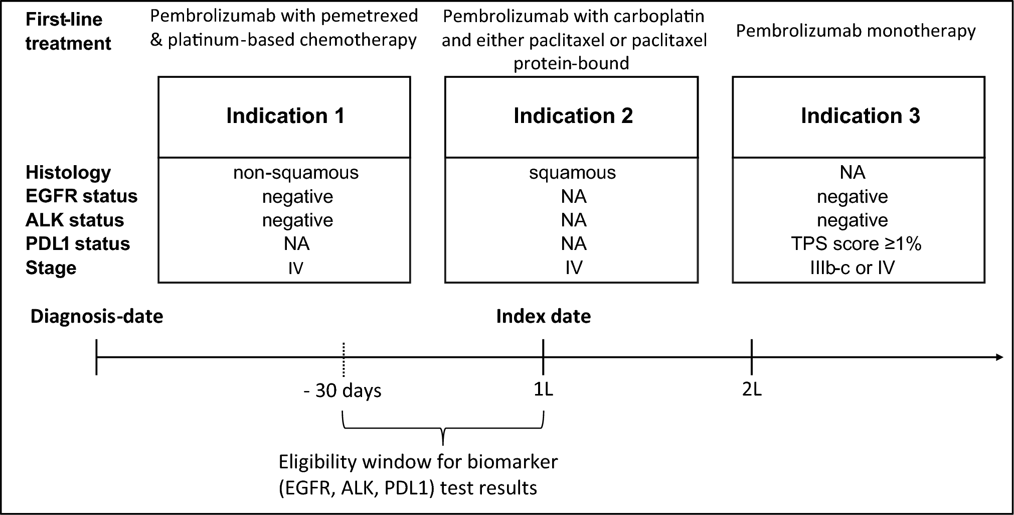
2.2 STM Structure

The model was built in Microsoft Excel® using a monthly cycle length modelled over a lifetime horizon (Fig. 1). The STM was structured to accommodate an OBA for tisagenlecleucel, using complete remission (response) at 3 months post-infusion as the clinically relevant outcome linked to payment. The CAR-T eligible population was captured using a decision tree to follow patients from the point of leukapheresis to assessment of response at 3 months; thereafter, patients entered the STM consisting of four health states: PFS, responder PD (RspPD), non-responder PD (NRspPD) and death. Patients who did not receive an infusion, due to an adverse event or manufacturing failure, were assigned to treatment with the comparator. Treatment initiation with blinatumomab was considered from the point of infusion, hence the entire patient cohort was modelled using three health states, PFS, PD or dead.

Fig. 1

State transition model structure with preceding decision tree for the CAR-T arm. CAR-T chimeric-antigen receptor T-cell therapy, PD progressive disease, PFS progression-free survival, STM state transition model

2.2.1 Transition Probabilities

Time-dependent transition probabilities for the health states were derived from sub-group analysis of pooled tisagenlecleucel data using event-free survival, referred to as PFS in the model, and OS time-to-event data. The transition probability for PFS to RspPD was calculated as the difference in the proportion of patients in event-free survival (EFS) from one cycle to the next, multiplied by the RspPD probability from the KM curve at the respective time point, and is described using the following equation:

$$\text= \left[(^\left(t\right)-^\left(t+1\right))\times ^\left(\text\right)\right]\times }_}$$

where SPFS is survival at time t from the EFS curve and SPD is survival at time t derived from the OS curve for patients who had responded at 3 months then lost response or progressed. PRsp is the proportion of patients in response at the time of entering the STM. To adjust for the event of death in calculating the proportion of patients in the RspPD state, background mortality was applied using standardised mortality ratio (SMR)-adjusted time-varying probabilities from Australian life tables. Tunnel states were used to track patients moving from PFS to RspPD so that time-dependent transition probabilities could be assigned. In other words, transitions in the RspPD state were dependent on the time since the last transition, without there being a change in the actual health state [9]. The transition probability for NRspPD to death was estimated from OS data for non-responders at 3 months. The proportion of patients in the death state for the entire cohort was calculated as 1 minus the sum of all patients alive, as described by the following equation:

$$_\left(t\right)=1-\left(_\left(t\right)_\left(t\right)+ _\left(t\right)\right)$$

where P is the proportion of patients in each health state at time t.

For blinatumomab, time in PFS was estimated by reconstructing individual data from the published KM OS curve [22], adjusted by a constant cumulative HR of 0.83 between OS and PFS [17]. Time-to-event data for blinatumomab patients moving from PFS to PD was not available, therefore transition probabilities for tisagenlecleucel NRspPD were applied. For the blinatumomab arm of the model, tunnel states were also used to apply time-varying transition probabilities to patients moving from PFS to PD.

2.2.2 Long-Term Survival

Long-term transition probabilities were derived by fitting parametric models to survival data for each sub-group. Selection of parametric model was based on whether the model was statistically a good fit according to the Akaike information criterion (AIC) and Bayesian Information Criterion (BIC), and also whether the extrapolated portion was clinically and biologically plausible [31]. Extrapolations were applied from the point on the KM curve where patient numbers were small (< 12 patients) due to a high level of censoring [32]. Long-term survival beyond 5 years ‘cure-point’ was extrapolated using a general mortality probability derived from Australian life tables. General mortality was adjusted by applying a standardised mortality ratio (SMR) of 9.05 from a Canadian cohort study in childhood cancer patients who had survived at least 5 years [24] to the proportion of patients remaining in PFS. Although no gradual transition was incorporated when switching from the extrapolated curve to an SMR-adjusted general mortality, the impact of different ‘cure-points’ on the ICER was tested in sensitivity analyses.

2.3 Partitioned Survival Model Structure

The model was built in Microsoft Excel® using a monthly cycle length modelled over a lifetime horizon. Consistent with the approach for the STM, the tisagenlecleucel arm included an initial decision tree to accommodate an OBA, followed by a series of PSMs dependent on the patients’ response status at 3 months. Unlike the STM, the proportion of patients who initially responded then progressed was estimated using AUC, calculated as the difference between the responder OS and PFS curves. Consistent with the STM approach, parametric models were used to extrapolate the observed data to year 5, after which SMR-adjusted all-cause mortality was applied. For the blinatumomab arm, a conventional three-health-state structure was applied with OS and PFS survival probabilities generated using the same approach as described for the STM.

2.4 Discrete Event Simulation Structure

Unlike the STM and PSM models, the DES model was developed using specialised software (Treeage Pro 2022, Williamstown, MA, USA) due to its computational complexity. The movement of patients through the model was determined by the probability of experiencing an event, randomly drawn from parametric time-to-event distributions [33, 34]. Unlike the STM and PSM approaches, the DES model explicitly included an infusion wait-time distribution for tisagenlecleucel, during which patients were at risk of manufacturing failure, a pre-infusion adverse event (AE) or death using probability distributions derived from different data sources. The model included a response assessment at 3 months to accommodate an OBA. The same data used for the STM was used to generate parametric probability distributions to calculate the time to event for patients in PFS and PD health states. Patients moved to a separate long-term health state at 5 years, where SMR-adjusted all-cause mortality was linked to individual patient age using bootstrapping. This meant that patients continued to remain in the health state in which they entered and were assigned the costs and QALYs from the relevant health, without moving to a progression state prior to death. For the blinatumomab arm, OS and PFS distributions were generated as described for the STM, although without access to individual patient data for blinatumomab, data for tisagenlecleucel non-responders were applied to patients in PD. Consistent with the approach for the tisagenlecleucel arm, patients alive at 5 years moved to a separate long-term health state where SMR-adjusted all-cause mortality was applied. In generating the base-case results, a total of 10,000 patient simulations were run. Additional simulations resulted in only minor changes to the results, by a matter of decimal places, with minimal impact on the ICER.

2.5 Utilities

The same utilities were applied to each model, with a pre-infusion utility applied to the DES model only. Utility values were calculated from patient-level EQ-5D-3L data from the ELIANA study using UK preference weights [35]. The PD state included EQ-5D assessments prior to infusion of tisagenlecleucel (while patients are in a progressive state) and after a PFS event, combined into a single PD utility. Utility data for patients prior to infusion with tisagenlecleucel was applied to the pre-infusion period in the DES. For blinatumomab, no published utility data were available, therefore tisagenlecleucel values were used. A one-off disutility was applied to each treatment arm to capture the loss of quality of life due to severe AEs including grade 3/4 cytokine release syndrome (CRS), other serious adverse events (SAEs) and subsequent SCT.

2.6 Costs

Cost inputs sourced from prior publications were adjusted for inflation using the Reserve Bank of Australia (RBA) inflation calculator [36], and when sourced from international publications, converted to Australian dollars (AUD) using RBA exchange rates [37]. All estimates of costs were calculated in AUD, although costs were reported in US dollars (USD), consistent with previous publications of the PSM and DES models [17, 38], using RBA exchange rates, April 2022 [37].The base case assumed a single payment of $375,000 for tisagenlecleucel at the point of infusion, converted from the NICE published price [25] as the Australian price is not publicly available. Costs associated with the administration of each treatment included the cost of leukapheresis, bridging chemotherapy (tisagenlecleucel only), cost of infusion, as well associated costs of managing serious AEs including tocilizumab for CRS and intravenous immunoglobulin (IVIg) for B-cell aplasia. The cost of SCT was included for the proportion of patients who received subsequent SCT in both the tisagenlecleucel and blinatumomab arms. The cost per course of blinatumomab was calculated using the Australian PBS price [26] as $49,127 (AUD 65,502) and an average number of treatment cycles from the clinical study [22], noting that the net price may be lower due to confidential pricing arrangements. In the DES model, treatment costs were applied as a one-off cost at the beginning of each decision node.

2.7 Model Assessment

A comparison of the models involved a quantitative assessment, in terms of costs, QALYs and the incremental cost-effectiveness ratio (ICER), and a checklist comprising the components captured by each model type, based on a set of parameters that affect the construction and outcomes of models for the cost effectiveness of CAR-T.

2.8 Quantitative Performance

Model traces were plotted to visualise the proportion of patients in PFS and PD over the first 5 years. Additionally, OS traces were graphed to assess any differences in the extrapolation of OS over a lifetime. Results were reported in LYs, QALYs and costs. Deterministic analysis was undertaken to test the impact of changes in CAR-T wait time, cure-point and duration of IVIg use as these parameters were considered uncertain due the lack of long-term data for CAR-T and in relation to CAR-T wait time, at risk of delay in clinical practice. The impact of removing the cure assumption completely so that extrapolation was independent of general mortality was also tested because previous studies identified greater differences in model results over the extrapolation period compared with the observed period [39, 40]. Additionally, sensitivity of the results to different OBAs was assessed by varying the rate of response at 3 months. Two different OBAs were tested, a split-payment arrangement (50% payment on infusion and 50% payment on response at 3 months) and a single payment on response only, using a weighted pricing approach so that the total cost for each OBA was equivalent to the base-case price of $375,000 for tisagenlecleucel, as described previously [17].

2.9 Checklist of Model Attributes

The components considered important in modelling the cost effectiveness of CAR-T were grouped into three categories pertaining to model flexibility, complexity and validity. Flexibility was defined as the ability to capture an OBA, incorporate CAR-T wait time and apply different long-term assumptions. Complexity was defined in terms of whether additional analysis of individual data was required, and validity in terms of the level of the concordance in the results generated.