Dataset

According to the theory in the classic classroom interaction observation and analysis system, such as Flanders Interaction Analysis System (FIAS) [38], nine types of behaviours captured through body movements and facial expressions are summarized from numerous behaviours. These behaviours include: accept, reject, ask questions, discussion, initiative talk, response, take notes/do exercises, lecture, and instruction. The dataset provides interactive sequences composed of multiple interactive behaviours and the duration of interaction occurring in a teaching scenario. These sequences showcase the dynamic process of behaviours in an interaction event, rather than isolated, irrelevant actions. They cover a variety of teaching scenarios such as Teacher Lecturing-Student Listening (01), Teacher Ordering-Student Execution (02), Q & A (03), and Group Discussion (04), with Group Discussion further divided into Student Discussion (51), Student-Teacher Group Discussion (52), and Teacher Discussion (53) sub-sequences.

We collected teaching videos from the Data Structures course (Project-Based Learning reform curriculum) at Beijing Normal University. Ten videos were randomly selected, in which discussion and lecturing segments were approximately equally represented, in order to obtain sufficient sequence and behaviour samples. These videos clearly record only the teacher’s voice, not the students. Each video was 45 min long, with a resolution of 1080 × 1920. In addition to 22–30 highly educated college students, several teachers participated: the head teacher stood at the podium, delivering lectures in Chinese using multimedia-assisted instructional design, while the other teachers sat at the back of the classroom, participating in group discussions and guiding students.

In the annotation process, experts first divided the entire teaching process into the four types of interactive sequences described above. Then, for each discussion sequence, they annotated each student group according to the three sub-sequences, in order to clarify the start and end times and the participants of each interaction process. It is important to note that there was no temporal overlap between two interactive sequences within the same video. Second, they manually annotated the interactive behaviours within each interactive sequence or sub-sequence. This included the behaviour category, start time, end time, actor index, actor identity (teacher or student), and location (upper-left corner coordinates (x, y), width, and height). Ultimately, we obtained 114 interactive-sequence samples, 332 sub-sequence samples, and 4,838 interactive-behaviour samples. These samples were divided into a training set and a test set at a ratio of 3:1, forming the BNU-SVIBD dataset.

Additionally, we evaluated the performance of our method on two public benchmark datasets that include interactive sequences and behaviours: the Volleyball dataset [39] and the Collective Activity dataset [5]. The Volleyball dataset [39] annotates 55 volleyball matches, containing a total of 3,493 training videos and 1,337 test videos. This dataset uses 8 sequence labels (right set, right spike, right pass, right winpoint, left set, left spike, left pass, and left winpoint) and 9 behaviour labels (‘blocking’, ‘digging’, ‘falling’, ‘jumping’, ‘moving’, ‘setting’, ‘spiking’, ‘standing’, ‘waiting’). The Collective Activity dataset [5] is annotated with everyday life scenes, consisting of 22 training videos and 12 test videos. This dataset uses 5 sequence labels (crossing, waiting, queueing, walking, and talking) and 6 behaviour labels (NA, crossing, waiting, queueing, walking, and talking).

Compliance with Ethical Standards

All students and teachers involved in the collected video signed informed consent forms. In terms of privacy protection, all annotators signed an agreement before the experiment, consenting not to share or modify the original complete videos. Additionally, we removed important personal information of the subjects, such as names, phone numbers, and contact addresses, from the database.

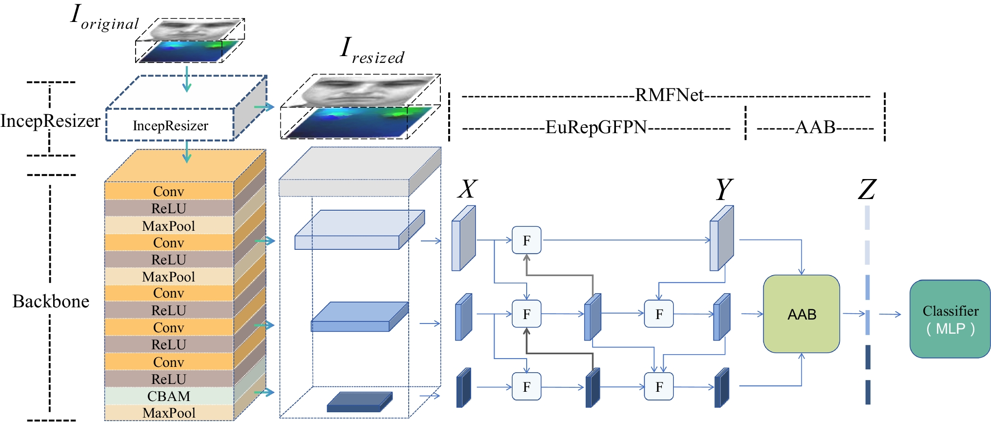
Implementation Details

All experiments were conducted on a single Corporation GA100 GPU with PyTorch. The image size of each frame was \(H\times\;W=1080\times\;1920\) and the maximum number of people captured was set to \(N=35\). The dimensions \(d\), \(_\), and \(_\) are 1024, \(_\times_\times1024\), \(_\times_\times1024\), respectively, where \(_\) indicates the total number of behaviour categories. The hyperparameters \(_=-3\) and \(_=2\). Our model was optimized using the Adam optimizer with \(_=0.9\) and \(_=0.999\), \(\text=^\). The weight decay was set to 0.2, and the learning rate was initially set to \(^\). One training of all data represented 1 epoch. In the actual training process, the number of epoch was 100, and the batch size was 2. The CNN used for feature extraction was RegNet-Y-32GF (as indicated in Fig. 3). Region features are extracted using RoIAlign with bilinear interpolation and a pooling size of \(5\times5\). The graph convolution layers in the model were set to 4.

Quantitative Analysis

To validate the effectiveness of our method, we quantitatively compared it with several state-of-the-art (SOTA) algorithms, including DIN [40], Improved ARG [29] and Decompl [41], on the proposed classroom interactive behaviour dataset. The experimental results, as shown in Table 1 (Ours), indicate that our method is superior to these algorithms. Among the other methods, the Improved ARG algorithm achieved the best overall accuracy, with 76.1% and 76.3% for interactive-sequence and behaviour recognition, respectively. In contrast, our method achieved 78.0% and 87.4% on these two tasks, corresponding to improvements of 1.9% and 11.1%. These results demonstrate that, by adopting causal intervention and the polyloss method [13], the proposed approach greatly improves the recognition accuracy of both sequences and behaviours.

Table 1 Experimental results on BNU-SVIBD

To further demonstrate the effectiveness of our method, we provide a comparison against state-of-the-art methods on public database, including Volleyball dataset and Collective Activity dataset. Since the behaviours in these datasets are difficult to obtain in other datasets, we did not assign weights to the temporal and spatial matrices. As shown in the Table 2, on the Volleyball dataset, our method achieved 94.8% activity recognition accuracy and 86.4% behaviour recognition accuracy. On the Collective Activity dataset, our method obtained 94.1% activity recognition accuracy and 80.7% behaviour recognition accuracy. The results outperform the state-of-the-art methods. This fully proves that eliminating confounding effects in both temporal and spatial dimensions and using the ployloss loss can effectively improve behaviour recognition performance.

Table 2 Experimental results on volleyball dataset and collective activity datasetAblation ExperimentMain Components Analysis

As shown in Table 3, to validate the effectiveness of the proposed method and its components, we designed ten sets of ablation experiments.

Table 3 Ablation study on BNU-SVIBD

First, to verify the effectiveness of the CRC module, we remove CRC and use only the IBC module to obtain the predictions. Without CRC (Ours-w/o CRC), the accuracy of interactive sequences and individual behaviour recognition drops from 78.0% to 69.8% and from 87.4% to 84.6%, respectively. This confirms that CRC plays a crucial role in inferring spatio-temporal dependencies between individuals.

Second, to evaluate the contribution of the polyloss method, we set all hyperparameters of the polynomial bases to zero. Without polyloss (Ours-w/o polyloss), the sequence and behaviour accuracies decrease to 77.1% and 86.9%, i.e., by 0.9 and 0.5% points compared with Ours. These results demonstrate that adjusting the weights of the polynomial bases according to different recognition tasks is indeed beneficial.

Third, to verify the effectiveness of assigning different weights to confounders, we set all confounder weights to a uniform value. With uniform weights (Ours-w same weight), the recognition accuracies for interactive sequences and behaviours decrease to 77.0% and 86.2%, which are 1.0 and 1.2% points lower than Ours. This indicates that allocating confounder weights based on educational activity statistics can effectively improve recognition performance.

Fourth, we verify the importance of the causal intervention module. Without causal intervention (Ours-w/o CI), the recognition accuracies decrease to 72.9% for sequences and 85.1% for behaviours, which means a drop of about 5 and 2.3% points, respectively. This shows that intervening on the spatio-temporal dependencies can effectively capture the causal relation from inputs to outcomes while reducing the influence of visual confounders.

To further examine the role of separating spatial and temporal disturbances, we conduct two additional ablations on the confounder dictionaries. When only spatial confounders are used (Ours-w/o t-confounder), the sequence and behaviour accuracies are 76.3% and 85.7%. When a single spatio-temporal confounder dictionary is adopted (Ours-w st-confounders), the accuracies further decrease to 75.9% and 85.9%. These results indicate that treating disturbances in the temporal and spatial dimensions separately yields better outcomes than using only one type of confounder or merging them into a single dictionary.

Fifth, we analyse the effect of the MGF module in the causal intervention head. When we replace MGF with a simple fully connected layer (Ours-w/o MGF), the sequence and behaviour accuracies drop to 77.2% and 86.3%, confirming that the multi-scale gated feedforward structure more effectively captures useful information in causal representations. To further understand the internal design of MGF, we consider three variants. When the multi-scale convolution paths are replaced by a single-scale convolution (MGF-single-scale), the sequence accuracy drops markedly to 72.3%, while the behaviour accuracy remains relatively high (86.4%). This suggests that rich multi-scale receptive fields are crucial for modelling complex interaction sequences. When we remove the multi-scale convolution branch and keep only the depthwise convolution branch (MGF-only-DWconv), sequence and behaviour accuracies are 75.0% and 86.8%. This indicates that the lightweight depthwise path alone is not sufficient to capture diverse spatio-temporal patterns, even though it can still preserve reasonable individual behaviour performance. In contrast, when we keep only the multi-scale convolution branch and remove the depthwise convolution branch (MGF-only-multi-conv), the sequence accuracy recovers to 77.8%, but the behaviour accuracy decreases to 85.8%, implying that the depthwise branch plays an important role in filtering noisy responses and preserving fine-grained behaviour cues. Taken together, these results show that both the multi-scale convolution paths and the depthwise gated branch are necessary, and their joint design in MGF provides a better balance between modelling capacity, noise suppression, and final recognition accuracy.

Stability Analysis

To further assess the stability of our model, we conducted experiments with five random seeds and quantified the variability of results across runs. Table 4 reports the performance on the BNU-SVIBD, Volleyball, and Collective Activity datasets for both activity recognition and action recognition, including the mean, standard deviation (Std), and 95% confidence interval (CI) over different seeds, thereby providing an intuitive view of the consistency and variability of the model’s performance. Overall, the mean results demonstrate that the model remains robust across all tasks and datasets. For example, on the BNU-SVIBD dataset for action recognition, the model achieves an average accuracy of 89.18% with a standard deviation of only 0.43%, indicating high stability under different random initializations.

Table 4 Performance under five random seeds (Mean ± Std, 95% CI)

To verify the statistical reliability of these results, we further report the 95% confidence interval (CI) for each task, which represents the range within which the true performance is expected to lie with 95% probability. All tasks exhibit narrow confidence intervals, suggesting that the model’s performance across runs is both stable and reliable. For instance, for activity recognition on the BNU-SVIBD dataset, the 95% CI is [76.47%, 79.13%], implying that performance fluctuations induced by different random seeds are minimal. Similarly, for activity recognition on the Volleyball dataset, the 95% CI of [94.30%, 96.06%] confirms that the model consistently maintains a high level of performance and is largely insensitive to the choice of random seed.

Robustness Analysis of the Literature-Based Prior Matrix

To verify the robustness of the literature-derived prior matrix \(}_\varvec}\), which is constructed from interaction patterns summarized in existing educational studies, we compare it with the data-driven prior matrix \(}_\varvec}^\varvec\varvec\varvec}\), obtained from the co-occurrence probabilities of behaviour pairs estimated on the BNU-SVIBD dataset. As reported in Table 5 (first row), the data-driven prior \(}_\varvec}^\varvec\varvec\varvec}\) achieves the best accuracy for individual behaviour recognition, while the literature-based prior \(}_\varvec}\) performs slightly better on the sequence-level task. This complementary trend indicates that the model does not rely on any single “gold-standard” prior; instead, any reasonable prior that captures the overall structure of teacher–student interactions is sufficiently effective. Both the data-driven prior \(}_\varvec}^\varvec\varvec\varvec}\) and the literature-based prior \(}_\varvec}\), can effectively capture similar patterns of behaviour co-occurrence, and the model performs well under either prior. Therefore, the CausalCIBR framework exhibits strong robustness to different sources of behaviour co-occurrence priors, whether derived from data or from literature. This also suggests that CausalCIBR can be broadly applied to classroom behaviour recognition tasks in different domains, without being tied to a specific educational setting or a particular body of literature.

Table 5 Comparison of model performance under different priors

Beyond directly comparing the data-driven prior \(_^\) and the literature-based prior \(_\), we further evaluate the robustness of CausalCIBR to prior misspecification by interpolating between \(_\)and a completely uniform prior. Specifically, we construct the following interpolated prior:

$$}_^}\left(\epsilon\right)=Normalize(\left(1-\epsilon\right)_+ϵU)$$

where \(\epsilon\in\\}\), and \(U\) is a uniform matrix representing a non-informative prior, i.e., all behaviour-pair co-occurrence probabilities are assumed equal. As shown in Table 5 (rows 2–8), when \(\epsilon=0.1\), the accuracy for interactive sequence recognition decreases, while the accuracy for behaviour recognition remains unchanged. This suggests that small prior errors have a certain negative impact on capturing interaction sequences, but only a minor effect on single-behaviour recognition. When \(\epsilon=0.2\) and \(=0.4\), although the accuracy of sequence recognition continues to decline, the accuracy of behaviour recognition actually improves. This may be attributed to a noise-enhancement effect, where moderate perturbations of the prior weaken mismatched or overly rigid prior assumptions, thereby amplifying certain discriminative behaviour features and enabling better recognition of individual behaviours. When \(=0.6\) and \(=0.8\), model performance degrades significantly, indicating that large prior deviations increasingly harm the model, especially in reasoning over behaviour co-occurrence patterns. At \(ϵ=1\), the prior becomes a fully uniform, non-informative prior. Although such a prior provides no guidance, it is unbiased; since it does not introduce any misleading structure, its performance is slightly better than that under the heavily mixed prior (\(ϵ=0.8\)). Overall, as \(\) increases, the prior bias gradually grows, yet the model is still able to maintain reasonably good performance within a certain range. This demonstrates that the CausalCIBR framework has a high tolerance to prior errors and can preserve relatively stable performance under various degrees of prior misspecification.

Robustness Analysis of the Confounder Dictionaries

To evaluate the robustness of the confounder dictionaries, we perturb the spatial confounder dictionary \(}_}\) and the temporal confounder dictionary \(}_}\)with Gaussian noise, and define the following perturbation process:

$$_^}=Normalize(_+\sigma\cdot\;N\left(\text\right))$$

$$_^}=Normalize(_+\sigma\cdot\;N\left(\text\right))$$

where \(\sigma\) denotes the perturbation strength, \(N\left(\text\right)\) is standard normal noise, and \(Normalize(\bullet)\) normalizes the perturbed dictionaries to ensure that their values remain within a reasonable range. By varying \(\sigma\) (i.e., the standard deviation of the injected noise), we simulate different levels of error in the confounder dictionaries. As shown in Table 6, when a perturbation of \(\sigma=0.1\) is applied separately to the temporal or spatial confounder dictionary (i.e., \(_^}(\sigma=0.1)\) and \(_^}(\sigma=0.1)\)), the model still achieves high accuracy, indicating that small noise perturbations have only a minor impact on performance. In this regime, the model can still effectively exploit the information encoded in the confounder dictionaries and remains stable.

Table 6 Experimental results of the confounder dictionaries under different perturbations

When \(\sigma=0.2\) for \(_^}\) and \(_^}\), the accuracy of interactive sequence recognition decreases and the accuracy of behaviour recognition also drops slightly, though the overall performance degradation is limited. This suggests that moderate errors in the confounder dictionaries begin to affect the model, especially for the more complex interactive sequence reasoning task. When the perturbation is increased to \(_^}\) and \(_^}\), the model performance degrades noticeably, particularly in terms of both interactive sequence recognition and behaviour recognition accuracy. This indicates that larger errors in the confounder dictionaries have a substantial negative impact on the model.

Overall, our method exhibits strong robustness to small perturbations of the confounder dictionaries and can maintain high performance under mild dictionary deviations. However, when the perturbation strength becomes too large—particularly when both the spatial and temporal confounder dictionaries are simultaneously corrupted—the model performance degrades significantly.

Adaptability and applicability analysis. To evaluate the adaptability of CausalCIBR across different classroom settings, we design two groups of experiments. The first investigates performance differences under varying group sizes based on people-density stratification (“People Density”); the second examines the model’s recognition ability under different interaction complexities based on behaviour-complexity stratification.

First, in the People Density experiment, we partition the samples into three groups according to the number of participants in the classroom scene: few people (5–9), medium (10–24), and many (25–35). As shown in Table 7 (rows 4–6), the model’s performance varies with group size. In low-density scenes with few participants (5–9 people), the interactive sequence recognition accuracy is 73.7%, while the individual behaviour recognition accuracy is relatively high at 89.6%. This indicates that in settings with fewer participants and relatively simple interaction chains, the model can more easily focus on and distinguish individual behaviours, whereas modelling complete interaction sequences remains somewhat challenging. By contrast, in medium-density (10–24 people) and high-density (25–35 people) scenes, the interactive sequence recognition accuracies reach 79.1% and 78.0%, and the individual behaviour recognition accuracies are 88.8% and 87.4%, respectively. As group size increases, occlusions, parallel interactions, and background distractions become more pronounced; nevertheless, CausalCIBR maintains high recognition performance, suggesting that the model can still capture useful spatio-temporal dependencies in more complex group interactions. Notably, within the medium-density range (10–24 people), the model achieves the best performance on both interactive sequence and individual behaviour recognition, reflecting a favourable balance between interaction complexity and the amount of observable information.

In the behaviour-complexity stratification experiment, we categorize behaviours into three types according to the number of participants involved and the strength of semantic dependencies: single-person behaviours (e.g., “take notes/do exercises”, “lecture”), two-person interactive behaviours (e.g., “ask questions”, “response”), and multi-person interactive behaviours (e.g., “discussion”, “instruction”). The results are also reported in Table 7 (rows 1–3). For single-person behaviours, the model attains an interactive sequence recognition accuracy of 77.0% and an individual behaviour recognition accuracy of 87.6%, indicating that CausalCIBR can reliably handle basic recognition tasks in scenes dominated by individual activities. For two-person interactive behaviours, the interactive sequence recognition accuracy reaches 77.1%, the highest among the three complexity levels. This suggests that the model can effectively characterise interaction patterns with explicit temporal dependencies—such as “question–answer” pairs—and capture the underlying causality and order structure between behaviours. In the multi-person interactive behaviour category, the individual behaviour recognition accuracy is 88.4%, the highest among all three categories. This shows that in complex interaction scenarios involving multiple agents and multi-directional information exchange, CausalCIBR can still extract highly discriminative behaviour representations from noisy and cluttered visual inputs.

Taken together, these two sets of experiments demonstrate that CausalCIBR maintains high accuracy in both interactive sequence and individual behaviour recognition across different group sizes and varying levels of behavioural complexity, evidencing strong contextual adaptability. On the one hand, the model can jointly model individual behaviours and overall interaction chains in classroom scenes ranging from low to high people density. On the other hand, along the gradient from single-person behaviours to multi-person interactions, the model likewise exhibits stable recognition performance. This adaptability primarily stems from the causal intervention mechanism on spatial and temporal confounders embedded in CausalCIBR. By explicitly introducing and intervening on the confounder dictionaries during spatio-temporal dependency modelling, the model is encouraged to learn causal relations that remain stable across different classroom configurations, rather than overfitting to high-frequency co-occurrence patterns specific to a particular scene. In other words, the disentangled representations approximate “distribution-agnostic” robust interaction patterns, enabling the model to retain relatively stable recognition performance under variations in both people density and behavioural complexity.

Causal Decoupling Capacity Analysis

In Causal CIBR, decoupling refers to the model’s ability to separate individual behaviour patterns and interaction relationships from spatio-temporal confounders (e.g., non-target students, background distractors, or events that frequently co-occur without genuine causal relevance). The goal is to ensure that behaviour and interaction predictions remain stable across different classroom layouts and people-density conditions. A better-decoupled representation should not only yield higher recognition accuracy, but also produce a confusion matrix with “sharper” class boundaries, exhibiting less entanglement between categories.

Table 7 Generalization results under different interaction complexities

To analyse which architectural components primarily govern the model’s causal decoupling capacity, we focus on the core modules that explicitly implement the causal pipeline: (1) The relation graph depth in the Causal Relation Construction (CRC) module (Graph_num), which determines the maximum length of interaction chains that the graph structure can represent; (2) The number of causal intervention steps (CI), which controls how many times the model uses the confounder dictionaries to adjust the spatio-temporal dependencies; (3) The number of MGF modules in the intervention head, which defines the model’s nonlinear capacity to separate causal semantics from residual confounding contexts under multi-scale receptive fields. Other components such as the backbone CNN and RoIAlign mainly affect the quality of generic visual features and are kept fixed in this analysis.

In addition to sequence-level and individual behaviour recognition accuracy, we introduce the confusion matrix entropy as an auxiliary metric for evaluating decoupling capacity. Concretely, we first normalize each row of the confusion matrix into a probability distribution over predicted classes, compute the Shannon entropy of each row, and then average over all classes. Lower entropy indicates that, given a ground-truth class, the predictions concentrate on a small number of labels, corresponding to sharper decision boundaries and reduced inter-class entanglement.

The experimental results are summarized in Table 8. When the number of graph convolution layers increases from 8 to 16 and 32, both sequence-level and individual behaviour recognition accuracies remain below the default configuration used in this work (Ours, with Graph_num = 4), and the confusion matrix entropy is generally higher (for example, the entropy is 0.60 when Graph_num = 16, compared with 0.53 for our model). This suggests that a moderate-depth relation graph already provides sufficient capacity to capture classroom interaction chains, while overly deep graphs tend to cause node features to become over-smoothed and to propagate noise, ultimately blurring the class boundaries.

Varying the number of intervention steps exhibits a similar pattern. When the number of CI layers is increased from the default of 1 to 2, 3, and 4, the sequence-level recognition accuracy decreases monotonically, the individual behaviour accuracy does not improve, and the confusion matrix entropy does not decrease accordingly. This indicates that a single causal intervention step is already sufficient to remove most harmful confounding effects; stacking additional intervention steps tends to over-regularize the representations rather than enhance the effective decoupling capacity.

By contrast, increasing the number of MGF modules mainly influences the model’s ability to distinguish fine-grained behaviour categories. Compared with MGF = 1, stacking more MGF modules markedly improves individual behaviour recognition accuracy (reaching up to 90.2% when MGF = 2), while keeping the confusion matrix entropy at a relatively low level (around 0.52–0.59). Sequence-level accuracy also improves slightly, reaching 78.6% when MGF = 4. These results indicate that the MGF modules provide scalable nonlinear capacity: they leverage multi-scale contextual cues to separate causal semantics from residual confounding context. However, the marginal gains diminish as the depth increases. In this paper, we adopt MGF = 1 as the default configuration to strike a favourable balance between accuracy, model complexity, and training stability; at the same time, the above results suggest that this component can be further scaled up when modelling richer behavioural vocabularies or more complex interaction patterns.

Overall, the experiments show that the decoupling capacity of CausalCIBR is not unbounded: its performance is primarily constrained by the expressive power of the MGF modules. In principle, increasing the number of MGF modules can support a larger set of behaviour classes and more complex interaction patterns; however, beyond a moderate depth, oversmoothing and over-regularization effects cause the performance gains to saturate or even degrade. In future work, we plan to explore adaptive hierarchical or multi-branch MGF architectures, which can dynamically allocate more capacity to interaction-dense scenarios and thereby further enhance the model’s ability to reliably decouple multiple behaviour categories and complex interaction chains.

Table 8 Results with different Graph_num, CI and MGF settings on BNU-SVIBDQualitative Analysis

To further verify the effectiveness of causal intervention, we visualized some example videos, comparing the recognition results using causal intervention (Ours) with those without causal intervention (w/o CI). By segmenting the videos by student groups and inputting them into the model for testing, we were able to showcase the interactive sequences and behaviours of the actors, as shown in Fig. 6. Due to issues such as multiple subjects, dense student targets, and severe occlusion in BNU-SVIBD, models without causal intervention are easily influenced by high-frequency categories such as “discussion”. Therefore, it is difficult to accurately construct spatio-temporal dependencies like “ask questions-response” or “discussion-accept”. Moreover, models without causal intervention also struggle to accurately capture interactive sequences, such as Q & A (03) stemming from behaviour relationships (e.g., “response-take notes/do exercises”). The proposed method, by intervening on weighted spatial and temporal confounders, accurately identifies interactive sequences and behaviours from the relationships between individual behaviours. This effectively overcomes the influence of visual confounders.

Fig. 6The alternative text for this image may have been generated using AI.

Qualitative results on BNU-SVIBD

Visualization-based Analysis of Model Components

To further analyse how each component of CausalCIBR contributes to behaviour recognition, we visualize the intermediate features on two representative classroom interaction sequences (Fig. 7). For each sequence, we show four stages of the processing pipeline: (1) backbone feature maps; (2) backbone + RoIAlign; (3) backbone + RoIAlign + Construct Actor Relation Graph (CARG) module; and (4) the final causal features after causal intervention (CI). Warmer colors (closer to red) indicate stronger activations, whereas cooler colors (closer to blue) indicate weaker activations.

In the backbone stage (first and sixth rows), the heatmaps mainly highlight high-contrast regions such as monitors, desks and chairs, tripod legs, and bright clothing. The activations spread over almost all students, including those not involved in the current interaction. This suggests that the CNN encoder tends to rely on frequently co-occurring contextual patterns and salient visual appearances rather than the actual interaction structure. At this point, the model cannot clearly distinguish which desks or which group of students are directly associated with the current label.

After adding the RoI features (second and seventh rows), the responses are constrained within the detected person bounding boxes, and background regions are strongly suppressed, leading to a substantial reduction in visual noise. However, multiple desks and student groups still receive comparable activation levels. At this stage, the model can already identify “who is present in the scene” and “where they are roughly located”, but it has not yet organized these individuals into interaction units or selected the key participants. In terms of network functionality, this stage mainly encodes individual actors and implicitly provides the basis for counting people and tracking their spatial positions.

Fig. 7The alternative text for this image may have been generated using AI.

Visualization of intermediate feature maps at four stages of CausalCIBR (backbone, backbone+ RoIAlign, backbone+ RoIAlign + CARG, and backbone+ RoIAlign + CARG + CI) on two representative classroom interaction sequences. Warmer colors indicate stronger activations, and cooler colors indicate weaker activations

When the relational graph (CARG module) is applied on top of the RoI features (third and eighth rows), the activation patterns become more structured. Nodes belonging to the same interaction group are strengthened, whereas isolated or distant students are down-weighted. For example, in both sequences, students around the main discussion table form a persistent cluster of strong responses, while students at other tables or in the back rows exhibit significantly weaker activations. This indicates that the RGC module is the core component that explicitly models the spatial layout and interaction relationships between participants: it effectively “counts” the people, organizes them into a graph structure, and propagates information along potential interaction edges.

The CI module further “rescues” those actors that are critical for behaviour recognition but were previously under-emphasized. In the visualizations, some independent interaction events—such as a teacher explaining beside a side desk or pointing to the screen to present their idea—show relatively low responses at the RGC stage, due to partial occlusion, proximity to the image boundary, or co-occurrence with a large-group interaction. After intervention, these regions appear clearly in yellow–red tones (high activation), indicating that the model now treats them as independent interaction chains rather than background. Meanwhile, students in the back rows and small-scale individuals in crowded scenes also exhibit notably enhanced activations. This behaviour highlights the core advantage of the CI module: by removing the influence of confounders on the target behaviours and strengthening responses to the target behaviours through multi-scale gated paths, it suppresses spurious co-occurrence patterns and amplifies those minority behaviours and interaction chains that are causally important but previously masked by dominant scene patterns.