Experiments are conducted on three widely used public datasets: SMIC [31], SAMM [29],and CASME II [30]. The SMIC dataset [31], released in 2013, contains 164 micro-expression samples from 16 participants, including 10 males and 6 females. This dataset is divided into sub-datasets such as SMIC-HS, SMIC-VIS, and SMIC-NIR. SMIC-HS samples were recorded using a high-speed camera at 100 frames per second (FPS), and they were labeled into three categories: positive, negative, and surprise. SMIC-VIS samples were collected with a regular camera at 25 FPS from 8 participants. In addition, samples were also recorded using a near-infrared camera and categorized into the SMIC-NIR. The SAMM dataset [29], released by the University of Manchester in 2018, consists of 159 micro-expression samples from 29 participants from different countries, covering 8 emotional categories: anger, happiness, other, surprise, contempt, disgust, fear, and sadness. The image resolution is 2024 × 1088. The CASME II dataset [30] was created by the Institute of Psychology, Chinese Academy of Sciences, in 2014, and contains 255 micro-expression samples from 26 participants, all of whom are Asian. It includes 7 basic emotional categories: other, disgust, happiness, repression, surprise, sadness, and fear. The image resolution is 640 × 480. The three-class experiments were conducted on the composite dataset MEGC2019 [37], which is composed of SMIC-HS, SAMM, and CASME II, as detailed in Table 2. The five-class experiments were conducted separately on the SAMM and CASME II datasets, with sample information provided in Table 3.

Table 2 Detailed information of the MEGC2019 datasetTable 3 Five-class sample information

In the five-class classification experiment, the Dlib library was used to crop and resize the apex frame images of the SAMM and CASME II datasets, and the optical flow maps were generated using the TV-L1 algorithm [38]. All experiments were conducted under the same configuration: Python version 3.12.3, PyTorch version 2.2.2 + cu121, NVIDIA 4060ti with 8GB of VRAM. The learning rate was fixed at 0.0005, and the batch size was set to 64.

Evaluation Metrics

This paper uses LOSO cross-validation for evaluation. The three-class classification task uses the Unweighted Average Recall (UAR) and Unweighted F1-score (UF1) as evaluation metrics, which are defined as:

$$UF1=\frac_^\frac_}_+F_+F_}$$

(10)

$$UAR=\frac_}^\frac_}_}$$

(11)

where \(C\) is the number of classes.\(T_\), \(T_\), \(F_\), and \(F_\) represent the numbers of true positives, true negatives, false positives, and false negatives, respectively, for class \(c\). \(_\) is the number of samples in class \(c\), and \(N\) is the total number of samples.

For the five-class classification task, the F1-score (F1) and Accuracy (Acc) are used as evaluation metrics, which are defined as:

$$Acc=\frac_^\left(T_+T_\right)}$$

(13)

where \(P=\frac_^T_}_^\left(T_+F_\right)}\) and \(R=\frac_}^T_}_^\left(T_+F_\right)}\).

All experiments used the CrossEntropyLoss function for training, with the following formula:

$$Loss=-\frac\sum_^\sum_^_\text(}_)$$

(14)

where \(_\) and \(}_\) represent the true label and predicted probability for the \(i\) -th sample in class \(c\), respectively.

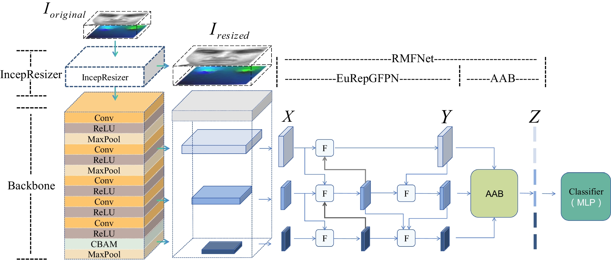
Ablation Experiments

To validate the effectiveness of different inputs, an ablation experiment, shown in Table 4, was conducted for the three-class classification. Since the optical flow contains motion information related, using the optical flow as input significantly outperforms using the apex frame as input. The apex frame contains texture information, which can complement the optical flow’s information. Therefore, the combined input can achieve optimal performance.

Table 4 The impact of different inputs

To validate the performance impact of each module, ablation experiments were conducted for the three-class classification. Table 5 records these models. To validate the effectiveness of the IncepResizer module, model A, B, and C, were conducted on MEGC2019. The results are shown in Table 6. Table 6 indicates that Model B outperforms Model A in both UF1 and UAR, suggesting that the Resizer module, compared to bilinear interpolation, can better retain task-relevant features. Further comparison between Model B and Model C shows that using Inception-v2 in Model C improves UF1 by 0.83% and 1.02% on the SMIC-HS and CASME II datasets, respectively, and improves UAR by 1.25% and 0.37%, respectively. However, on the SAMM dataset, UF1 and UAR decrease by 1.13% and 0.36%, respectively. Although there are fluctuations on certain datasets, the overall performance improvement verifies the IncepResizer module’s feasibility.

Table 5 Details of the three-class ablation experiment modelTable 6 IncepResizer module validation

To validate the effectiveness of the EuRepGFPN module, models C and D were conducted and the results are shown in Table 7. We can see that the model using EuRepGFPN (Model D) outperforms the model using RepGFPN (Model C). In particular, on the SAMM dataset, Model D achieves a 9.18% and 11.09% increase in UF1 and UAR, respectively, compared to Model C. This demonstrates that the EuRepGFPN module enhances the interaction of multi-scale features by optimizing upsampling, further improving the overall performance of the model. From Table 8, we can see that the CBAM module with a convolution kernel size of 7 is more suitable for the current task. On the MEGC2019 dataset, Model F (K = 7) outperforms Model D (without CBAM enabled) by 1.62% and 0.13% in UF1 and UAR, respectively. This demonstrates that the CBAM module can enhance key features through the attention mechanism, improving the model's performance.

Table 7 EuRepGFPN module validationTable 8 AAB module validation

Besides we compare the impact of different levels of dimensionality reduction on model performance. Detailed parameter settings are shown in Table 9.\(}\),\(}\), and \(}\) represent the convolution kernel size, stride, and padding, respectively. \(}\) and \(}\) represent the target height and width for adaptive average pooling, while"—"indicates that the corresponding processing is not applied.

Table 9 Different dimensionality reduction methods

The experimental results in Table 10 indicate that using Method 2 for dimensionality reduction achieved the best classification performance. This suggests that excessive dimensionality reduction may result in information loss, preventing the model from effectively capturing key information. On the other hand, insufficient dimensionality reduction may lead to feature redundancy, increase computational complexity, and even cause overfitting.

Table 10 The impact of different dimensionality reduction methods

Different settings of the repetition count (n = 1,2,3,4,5) for the BasicBlock inside the FusionBlock were tested. The results are shown in Table 11. The results indicate that the repetition count of BasicBlock has a significant impact on model performance. When the repetition count n = 3, the recognition performance was optimal, and the model achieved the best performance.

Table 11 The impact of BasicBlock repetitions

Different settings of the repetition count (n = 1,2,3) for IncepResBlock in the IncepResizer module were tested. The results are shown in Table 12. When n = 2, the model performance reached its best. On the MEGC2019 dataset, the UF1 of the n = 2 model was improved by 2.55% and 2.19% compared to the n = 1 and n = 3 models, respectively. The UAR of the n = 2 model was improved by 1.89% and 2.03% compared to the n = 1 and n = 3 models, respectively.

Table 12 The impact of IncepResBlock repetitions

As shown in Fig. 12, PT is strongly influenced by the perturbation intervals \(\Delta }\), where excessively high or low perturbation frequencies both fail to yield optimal performance. Smaller intervals result in overly frequent perturbations, which disrupt the model’s normal fitting process; conversely, the larger intervals produce perturbations that occur too infrequently to drive the model away from its reliance on local features, thereby limiting the expected improvement in generalization. Based on these observations, we set the perturbation interval to be 20.

Fig. 12The alternative text for this image may have been generated using AI.

The effect of perturbation intervals \(\Delta }\)

As shown in Fig. 13, the effects of each data augmentation operation are different when used individually, and the improvement is limited. Among them, the effects of color jitter and random masking are noticeably lower than the other two operations. However, we still believe that color jitter and random masking are crucial components of a comprehensive data augmentation strategy, as they are irreplaceable in simulating lighting changes and occlusion. When multiple augmentation operations are combined, they can generate more diverse samples, leading to better overall gains.

Fig. 13The alternative text for this image may have been generated using AI.

Independent ablation of different data augmentation operations (GJ represents color jitter, GN represents gaussian noise, HF represents horizontal flipping, RM represents random masking, ALL represents the simultaneous application of all four operations)

To validate the effectiveness of perturbation training (PT), tests were conducted on HTNet and RRMFNet using PT. The results are shown in Tables 13 and 14. Table 13 shows that in the three-class classification task, the models using PT performed better. On the MEGC2019 dataset, the UF1 and UAR of RRMFNet + PT improved by 0.45% and 1.01%, respectively, compared to RRMFNet without PT. Particularly on the CASME II dataset, the UF1 and UAR of RRMFNet + PT improved by 1.81% and 2.09%, respectively. The UF1 and UAR of HTNet + PT on the MEGC2019 composite dataset improved by 1.3% and 1.91%, respectively, compared to HTNet. Table 14 shows that in the five-class classification task, PT also exhibited excellent performance. On the SAMM dataset, the F1 and ACC of RRMFNet + PT improved by 8.45% and 5.15%, respectively. On the CASME II dataset, the F1 and ACC of RRMFNet + PT improved by 5.28% and 3.65%, respectively. It is evident that the PT strategy significantly enhances the model's generalization ability.

Table 13 The impact of PT on the three-class classificationTable 14 The impact of PT on five-class classification

The confusion matrix comparison in Figs. 14 and 15 shows that the PT strategy has a significant effect on balancing classification, effectively alleviating the impact of small sample problems and class imbalance. Particularly for the classes with scarce samples, the improvement effect of the PT strategy is more pronounced.

Fig. 14The alternative text for this image may have been generated using AI.

Three-class confusion matrix. The upper row (a, c, e, g) presents the outcomes prior to the introduction of PT, whereas the lower row (b, d, f, h) depicts the outcomes subsequent to the introduction of PT

Fig. 15The alternative text for this image may have been generated using AI.

Five-class confusion matrix: The left side (a, c) shows the results before introducing PT; the right side (b, d) shows the results after introducing PT

However, for categories with extremely scarce samples, the improvement effect of the PT strategy has certain limitations. For example, in the three-class experiment on the SAMM dataset, although the PT strategy overall improved the model's classification performance, the recognition rates of the Positive and Surprise categories remained relatively low. Similarly, in the five-class experiment on the SAMM dataset, although the PT strategy generally improved the model's classification performance, the recognition rates of the Contempt and Others categories were still low. This may be related to the relatively small number of samples in the corresponding categories, weak feature representation, and significant feature overlap with other categories in the SAMM dataset.

Comparison with Other Methods

To validate the superiority of the proposed algorithm, we conducted comprehensive experiments shown in Table 15. The results indicates that the overall performance of RRMFNet + PT achieved the optimal level in the three-class classification task. RRMFNet + PT improved UF1 and UAR by 2.86% and 0.83%, respectively, compared to the sub-optimal method, SRMCL, on MEGC2019. On the SMIC-HS subset, RRMFNet + PT improved UF1 by 3.67% compared to the sub-optimal method, HTNet. On the SMIC-HS subset, RRMFNet + PT improved UAR by 5.23% compared to SRMCL. On the CASME II subset, RRMFNet + PT improved UF1 and UAR by 1.29% and 1.43%, respectively, compared to SRMCL. However, on the SAMM dataset, the UF1 of the proposed algorithm is 2.24% lower than that of OFF-ApexNet, and the UAR is 4.83% lower than that of SRMCL. The possible reasons are the obvious data imbalance issue on the SAMM dataset: the proportion of "negative" samples accounts for 69.17%, while the proportion of "surprise" samples is only 11.28%. As can be seen from Figs. 14(c) and (d), the perturbation strategy can improve the recognition accuracy of few-shot categories to a certain extent, but at the same time, the recognition accuracy of the "negative" category slightly decreases. In addition, the samples in the SAMM dataset also have racial differences and a large age range (19–57 years old), while the proposed algorithm does not involve relevant modules to eliminate the negative impact of these differences on expression recognition. This issue may also be related to the adaptability of the model architecture, thus leading to a decline in the performance of the algorithm on this dataset.

Table 15 Three-class comparison

The five-class classification task was compared with related algorithms in the last six years. The results are shown in Table 16. We can see that the overall performance of RRMFNet + PT also achieved the optimal level in the five-class classification task. RRMFNet + PT improved ACC by 1.55% compared to the sub-optimal method, SGTRCN-G, on the SAMM dataset, and the F1 score reached the sub-optimal level. On CASME II, RRMFNet + PT improved F1 by 9.13% and improved ACC by 3.51% compared to SGTRCN-G. In particular, the RRMFNet + PT method still exhibits limitations on the SAMM subset. In the five-class classification task, RRMFNet + PT’s F1 is 3.07% lower than SGTRCN-G. In the five-classification task, the SAMM dataset also exhibits more pronounced class imbalance compared to the CASME II dataset, and the experimental results show that the contempt category is often misclassified as the others category. Specifically, the classification performance for contempt and others categories is weaker. These issues may be attributed to class imbalance, insufficient inter-class differences, and the mismatch of the model architecture.

Table 16 Five-class comparisonComplexity Analysis of the Model

Since computational cost is crucial for model deployment, we compare the computational consumption of RRMFNet with HTNet and SRMCL, as listed in Table 17. Results in Table 17 indicate that in terms of parameters, RRMFNet has 43.7M parameters, which is significantly lower than HTNet’s 139.5M (a reduction of approximately 68.6%) and substantially less than SRMCL’s 329.2M (a reduction of around 86.7%), demonstrating obvious advantages in model storage overhead. Regarding computational complexity, RRMFNet achieves 5.9G FLOPs, which is notably higher than HTNet’s 214.3M (about 27.5 times that of HTNet). This results in higher requirements for inference speed and hardware resources, making RRMFNet relatively more difficult to deploy and requiring more cautious adaptation in resource-constrained devices or scenarios. However, in terms of performance, RRMFNet achieves 2.68% and 3.37% improvements in UF1 and UAR on the MEGC2019 composite dataset compared to HTNet. Compared with the 64.8G FLOPs of SRMCL, our RRMFNet drastically reduces computational cost to only 9.1% of that. Furthermore, it achieves improvements of 2.86% in UF1 and 0.83% in UAR on the MEGC2019 dataset, striking a favorable balance between “low complexity” and “high performance”. In summary, compared with HTNet and SRMCL, RRMFNet’s core advantages lie in the substantial reduction of parameters and steady performance improvement. However, it should be objectively noted that its FLOPs are significantly higher than those of the lightweight model HTNet, leading to a relatively higher deployment threshold. Thus, the selection should be based on the resource conditions of specific application scenarios.

Table 17 Model computational consumption comparison

We also conducted experiments to evaluate the parameter distribution across each module, as summarized in Table 18. The results indicate that EuRepGFPN, which serves as the core module of RRMFNet, contributes the largest portion of parameters in our method. Given that the complete model cannot function without EuRepGFPN, its computational cost (FLOPs) is primarily assessed through Table 19. Our analysis shows that discarding modules such as AAB without CBAM and IncepResizer only slightly reduces the overall FLOPs, confirming that EuRepGFPN accounts for the majority of computational complexity.

Table 18 Parameters of each moduleTable 19 Evaluation of computational cost