LAPNN Model Overview

Human cyber physical networks (HCPNs) in the proposed model are complex sociotechnical networks of human, cyber, and physical agents interacting at different hierarchy layers within an industrial context. In practice, these agents can be implemented as digital twin nodes interconnected through industrial, IoT, or publish-subscribe protocols. They are therefore represented in the cyber domain as LAPNN nodes, and their communication channels as mechanistic or structural links. (see Fig. 1).

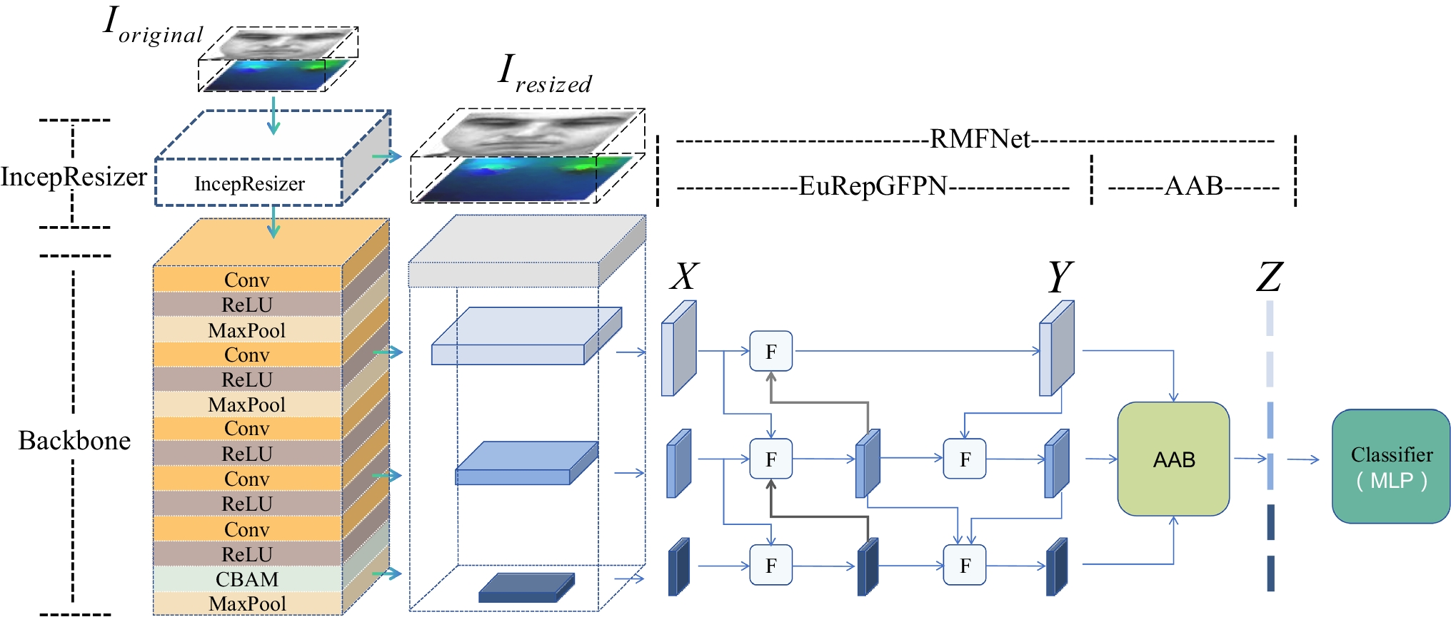
The LAPNN performs cognitively inspired analogical-style reasoning in four sequential stages, summarized here and illustrated in Fig. 2(a–d):

1.

Description Semi-stable spatio-temporal motifs are extracted from observed time-varying feature dynamics and encoded as composite sparse binary distributed representations (SBDRs), producing a symbolic description of the observed structure.

2.

Retrieval The encoded motif is used as a probe to retrieve the most similar previously learned motif from associative memory.

3.

Mapping Node-level representations associated with the retrieved motif are recalled and greedily mapped to the nodes of the newly extracted motif, allowing structural misalignments to be corrected.

4.

Inference Part–whole (graph-level) and is-a (node-level) inference are carried out, and the resulting symbolic node representations are decoded back into numeric feature and matrix column vectors.

Fig. 1The alternative text for this image may have been generated using AI.

Hierarchy of human–cyber–physical networks (HCPNs) in an industrial context. Agents at multiple levels interact via structural cyber links

Fig. 2The alternative text for this image may have been generated using AI.

Overview of the LAPNN model. Panels (a–d) show the four stages of processing: (a) motif extraction, (b) encoding, (c) analogical-style motif retrieval and node mapping, and (d) part–whole and is-a inference with decoding of node representations

Structural Motif Extraction

Let \(G=(N,E)\) be a universal graph constructed from an observed industrial task or a collection of tasks. The set of nodes N is associated with features F, comprising both static attributes, such as class or instance, and time-varying signals, including spatial position and sensor states. These features are sampled over T time steps within one or more execution cycles of the task. Each node is indexed in the order observed and keeps this as a pool index for furture ordering of motif nodes.

To establish structural relationships in a sliding window w, the time-varying node signals are aggregated into a scalar quantity or a representative signal is selected to serve as a base correlation feature \(v_i(t)\). Pairwise correlations between node signals are computed while accounting for temporal lags, creating a correlation matrix \( \textbf \in \mathbb ^ \).

To emphasize human-centrism in human–cyber–physical systems, a human weighting parameter \(\lambda _h\) is applied to correlation entries involving human-grounded nodes. Correlation values exceeding a threshold \(\tau _\) define directed structural adjacency matrix \( \textbf \in \mathbb ^ \), as well as edges between nodes, whose weights are human-biased correlation values.

Over sequences of sliding windows, the establishment and decay of these edges gives rise to spatiotemporal motifs that characterize recurring spatial and temporal relationships among system components for a given industrial production task. In the absence of sustained correlation, edges gradually attenuate, while repeatedly reinforced connections persist, leading to motifs that are neither static nor transient. This behavior is analogous to the formation and pruning of structural connections indirectly observed in spatiotemporal brain imaging, such as fMRI, where anatomical connectivity patterns emerge and recede over time with use or neglect [7]. A motif M defines a single HCPN corresponding to a given industrial task, and provides the structural substrate to be subsequently encoded into a symbolic description by the LAPNN. See Fig. 2(a).

Node and Motif Encoding in Associative Memory

An extracted motif M consists of m nodes ordered by their node pool indices and a directed adjacency matrix \(\textbf_M \in \mathbb ^\). To preserve temporal flow while ensuring real-valued spectra, we construct a directed graph Laplacian adapted from [44],

$$\begin \textbf_M = \textbf - \tfrac \left( \varvec^ \textbf \varvec^ + \varvec^ \textbf^\top \varvec^ \right) , \end$$

(1)

$$\begin \textbf = \textbf_}^ \textbf_M, \end$$

(2)

where \(\varvec=\textrm(\varvec)\) and \(\varvec\) is the stationary distribution of the random walk defined by \(\textbf\). The eigenvectors of \(\textbf_M\) are sorted by increasing eigenvalue magnitude. The directed Laplacian provides a principled spectral descriptor for spatial and temporal interaction graphs; a systematic comparison with alternative message-passing mechanisms is left to future work.

Each node \(i \in M\) is associated with three numeric vectors: the adjacency column \(\textbf_i\), the Laplacian eigenvector \(\textbf_i\), and a static context feature vector \(\textbf_i\). These are encoded into sparse binary distributed representations (SBDRs) of fixed dimensionality d using role–filler binding with additive context-dependent thinning (CDT) [50].

For a numeric vector \(\textbf \in \mathbb ^k\) (either \(\textbf_i\) or \(\textbf_i\)), each element \(x_j\) is mapped to a filler SBDR via a numeric encoder \(\psi _n(x_j)\) adapted from [51], and bound to a positional role SBDR \(\psi _r(j)\). All bound elements are aggregated using CDT to form a composite representation, denoted \(\hat}_i\). Static categorical features \(s_\) are similarly encoded using random role vectors \(\psi _r(s_)\), producing a composite static context representation \(\hat}_i\).

Given these components, the final SBDR representation of node i is defined as

$$\begin \textbf_i = \text \!\left( \hat}_i, \hat}_i, \hat}_i \right) = \left\langle \hat}_i \vee \hat}_i \vee \hat}_i \right\rangle . \end$$

(3)

To enforce human-centrism, the representations of nodes within a motif are pooled in a designated human node operating at the hierarchy level \(\ell - 1\), yielding a composite representation at level \(\ell \) (Fig. 2c). The pooled motif representation is

$$\begin \textbf^ = \left\langle \textbf_1 \vee \textbf_2 \vee \dots \vee \textbf_m \right\rangle . \end$$

(4)

Analogical-Style Retrieval

Given a pooled motif representation \(\textbf^\) extracted from an observed HCPN motif at hierarchy level \(\ell - 1\), the LAPNN performs analogical-style retrieval to identify a previously learned motif representation with similar structure. Retrieval is carried out by the operator \(\Gamma _r\), which probes the associative memories of LAPNN nodes having representations at level \(\ell \), using \(\textbf^\) as a probe vector.

Each LAPNN node maintains its own associative memory, internally organized into representation levels. If a node maintains a pooled representation, this representation resides in the node’s associative memory at the corresponding internal level. Human-grounded nodes at the lowest hierarchy level (\(\ell = 0\)) do not maintain pooled motif representations and therefore do not participate in motif-level retrieval.

Let \(\mathcal _v^ = \_^, \dots , \textbf_^\}\) denote the set of pooled motif representations in the associative memory of LAPNN node v. Retrieval selects the most similar stored motif according to a similarity measure \(\textrm(\cdot ,\cdot )\) in SBDR space:

$$\begin \textbf'^ = \Gamma _r\!\left( \textbf^\right) = \arg \max __^ \in \mathcal _v^} \textrm\!\left( \textbf^, \textbf_^\right) . \end$$

(5)

The motif representation retrieved \(\textbf'^\) serves as an analogical structural template, allowing the recall of associated node representations.

Node Recall and Greedy Mapping

After a composite motif representation \(\textbf'^\) has been retrieved by \(\Gamma _r\), it is used as a probe to recall the set of node representations associated with that motif. This recall is performed by probing the LAPNN node pool using a top-k similarity retrieval in SBDR space, yielding a candidate set of recalled node representations \(\'_j\}_^\) belonging to the retrieved motif.

To establish a correspondence between the observed motif \(\_i\}_^\) and the recalled motif \(\'_j\}_^\), the LAPNN performs greedy node mapping using the operator \(\Gamma _m\). Each observed node representation \(\textbf_i\) is compared against all currently unmatched recalled node representations \(\textbf'_j\) using a similarity measure in SBDR space. The recalled node with the highest similarity score is selected as the match for \(\textbf_i\), after which both nodes are removed from further consideration. This process is repeated until all observed nodes are mapped or no viable matches remain.

The similarity scores computed during this procedure can be interpreted as forming an \(m \times p\) similarity matrix, where m and p are the orders of the observed and retrieved motif graphs, respectively. Greedy mapping corresponds to iteratively selecting the maximal entry in this matrix and masking the corresponding row and column.

Importantly, because node representations are composed using role–filler bindings with SBDRs, positional information is encoded in a graded manner, rather than as a hard index. As a result, a node that occupies position i in the retrieved motif may exhibit a high similarity to a node that occupies position \(j \ne i\) in the observed motif. This property enables the LAPNN to tolerate structural misalignment and still recover meaningful correspondences, allowing analogical transfer across human subjects, task executions, or sensing configurations with differing node orderings (see Fig. 2(d)).

Inference and Decoding

Once a motif representation has been retrieved from associative memory, both graph- and node-level tasks can be carried out via associative recall. Composite SBDRs, such as the pooled motif representation \(\textbf^\), can be clustered by similarity, allowing structural or semantic retrieval. Any role or context can be bound to these representations using CDT during encoding and similarly separated during inference.

For example, given a retrieved motif \(\textbf^\) and a role SBDR \(\textbf_c\) encoding a context vector \(\textbf\), the approximate context component \(\tilde}\) can be isolated using

$$\begin \tilde} = \langle \textbf^ \vee \textbf_c \rangle \wedge \lnot \textbf^, \end$$

(6)

where \(\langle \cdot \rangle \) denotes the additive CDT operation and \(\lnot \) is the bitwise complement.

The decoding of a node representation is then performed by isolating its constituent SBDRs and mapping them back to their numeric or categorical values:

$$\begin \text \!\left( \hat}_i, \hat}_i, \hat}_i \right) , \end$$

(7)

recovering the adjacency, eigenvector, and static feature information from the encoded SBDRs. This enables both is-a node-level classification and part-whole graph-level motif inference, without relying on gradient-based learning and taking advantage of the associative memory of the LAPNN for brain-inspired analogical-style reasoning and generalization.

Training and Memory Update Mechanism

The LAPNN does not rely on backpropagation. Instead, it uses a gated memory consolidation mechanism based on loss-improvement. The combined loss for a single motif is defined as the mean of the graph-level and node-level losses, where the loss is calculuated on the attempt to recall a graph or node from the current associative memory, rather than on a validation set:

$$\begin \mathcal _}&= \frac \Big ( \mathcal _} + \mathcal _} \Big ). \end$$

(8)

For each structural motif M, the LAPNN node associative memory update is gated, where an encoded motif representation is stored in associative memory only if its combined current loss exceeds a minimum threshold \(\tau _}\) and improves the best previously observed loss:

$$\begin \text (m, t)&=\mathbb \Big [\tau _}< \mathcal _}^(t) < \mathcal _^(t) \Big ],\end$$

(9)

$$\begin \mathcal _^(t)&= \min _ \mathcal _}^(t'), \quad \mathcal _^(0) = +\infty . \end$$

(10)

This mechanism ensures that only representations that reflect meaningful learning progress are consolidated while suppressing both noisy and trivial updates. Each motif tracks the minimum combined loss observed up to the current time step, initialized to \(+\infty \) so that the first valid observation is always admissible for memory storage.

Crucially, this approach supports continuous incremental learning. As new observations and human subjects are introduced, the model updates its associative memory without retraining network parameters. This enables rapid adaptation in human–robot collaboration scenarios and other HCPS applications, reflecting one of the key advantages of the LAPNN for continuous learning with minimal data.

Dataset and Task Definition

The experiments were conducted on a modified version of the Collaborative Action (CoAx) dataset [23], which contains multimodal recordings of six human subjects performing three industrial tasks, including a human–robot collaboration scenario. Each subject performed multiple takes per task, resulting in repeated executions with natural variation in motion and timing.

A computer vision pipeline was used to process image frames and classify detected entities into semantic categories such as human, right hand, screwdriver, and other task-relevant objects. For each frame, 3D bounding boxes and associated metadata were extracted and stored in a structured directory structure.

Each task execution (take) consists of a sequence of T frames, indexed by \(t = 1, \dots , T\). For each frame t, a set of N node objects is observed, corresponding to human, cyber, and physical entities present in the scene (e.g., human, hands, tools). One take out of ten was pseudorandomly selected, after which object centroids were estimated from the bounding box information, and velocities were computed from position differences across consecutive frames.

The resulting node feature set combines continuous kinematic attributes with categorical context information and is defined as

$$\begin F = \_x,\; \text _y,\; \text _z,\; \text ,\; \text _},\; \text _},\; \text _},\; \text _}\}. \end$$

(11)

The tasks were defined as 1) graph-level classification for predicting which industrial collaborative task an observed motif or graph belongs to, and 2) node-level classification, predicting which object class a given node represents. The tasks are carried out by masking class and instance features in the data. Given a partially observed graph, we sought to determine whether a model could predict which task is being carried out, and whether it could recover the missing (masked ) semantic labels of nodes.

Baseline Model and Comparison Framework

We chose the Temporal Heterogeneous Graph Neural Network (THGNN) proposed by Wen, Fang, Wei, Liu, Chen, and Wu [15] as a baseline due to its focus on learning spatiotemporal relational structure in heterogeneous industrial systems. Unlike many other GNNs, which typically operate on fixed graph structure, the THGNN infers dynamic dependencies from multivariate time series using a FiLM-based hypernetwork and has demonstrated strong performance in graph-level industrial inference tasks. This choice of the THGNN, with its FiLM hypernetwork, represents a contemporary benchmark for spatiotemporal, heterogeneous graph learning. In this paper, we demonstrate that the LAPNN is not only comparable to this state-of-the-art method in graph classification but also offers more efficient generalization to unseen human subjects and enables associative node recall — a feature missing in typical global-pooling architectures.

Since no official implementation was available, we reimplemented the baseline model following the description in the original work. The THGNN was originally proposed for graph-level RUL regression; we adapted it to graph-level classification by replacing the regressor after the pooling layer with a classification head, and by adding an auxiliary node-level classifier as a diagnostic probe of node-level information in the learned representations, while keeping the remaining architecture unchanged.

We tested a simple MLP on the THGNN FiLM embeddings for each node to determine whether node identity could be inferred. Using the outer split with the highest observed node F1, the MLP achieved a mean ± std node F1 of 0.071 ± 0.042. These results were used to verify the feasibility of auxiliary node classification using the THGNN’s learned representations.

The LAPNN extracts structural motifs using velocity features to infer graph connectivity, with static node context features used for representation learning and during associative inference. In contrast, the THGNN uses position, velocity, and static node context features jointly, for graph relation inference in the FiLM module, and for message passing during embedding learning.

At the graph level, the LAPNN and THGNN were compared in their ability to classify the industrial task corresponding to the extracted motif embedding or constructed representation. Node-level classification is native to the LAPNN through its associative recall mechanism. While our reimplementation of the THGNN also supports auxiliary node-level classification, it is not explicitly optimized for node-level tasks, and does not enforce preservation of node identity in its latent representations.

Both models were evaluated with identical data splits and probability of feature masking. In the LAPNN, static features \(\text _\), \(\text _\) were masked in the observed motif representation with just their structural components visible, whereas in the THGNN, those input features were masked as the embeddings were generated for the observed graph. Each model then attempted to classify the resulting partial node representation. While the masked feature subsets were not identical, both models employed the same masking probability (\(p=0.1\)), ensuring comparable levels of partial observation.

Cross-Subject Incremental Evaluation

We used an adaptation of the the nested cross-validation protocol of [52] to an incremental learning setting, where model parameters and memory items were retained as additional human subjects are introduced. The objective was to estimate generalization performance on an unseen human subject and then analyze scaling with more training subjects.

Let \(\mathcal = \\) denote the set of subjects, with data \(\mathcal _s\) for subject s. An incremental learning algorithm is defined as

$$\begin f_,\pi } : \bigl ( \mathcal _, \dots , \mathcal _ \bigr )&\mapsto \hat, \end$$

(12)

where \(\varvec\) denotes hyperparameters and \(\pi \) a subject curriculum.

Outer Loop (Leave-One-Subject-Out)

For each test subject \(s^ \in \mathcal \),

$$\begin \mathcal _}&= \mathcal _}, \end$$

(13)

$$\begin \mathcal _}&= \mathcal \setminus \\}. \end$$

(14)

For each sampled curriculum \(\pi \in \Pi (\mathcal _})\), the model was trained incrementally and evaluated on \(\mathcal _}\). During a post-hoc analysis of the resulting scores, training was considered complete if

$$\begin \textrm_} \ge \tau _}, \end$$

(15)

with \(\tau _} = 0.95\).

For each test subject

Inner Loop (Hyperparameter Selection)

Given candidate hyperparameters \(\_1,\dots ,\varvec_K\}\), validation was performed by selecting \(s_} \in \mathcal _}\) and training on \(\mathcal _} \setminus \}\}\). Selection was driven by the composite metric

$$\begin \mathcal _}(\varvec)&= \lambda \cdot \textrm_} + (1 - \lambda ) \cdot \textrm_}, \end$$

(16)

yielding

$$\begin \varvec^ = \arg \max __k} \mathbb \!\left[ \mathcal _}(\varvec_k) \right] . \end$$

(17)

The specific search space for these hyperparameters, including the LAPNN correlation threshold for motif extraction, as well as the THGNN layer dimesnions, is summarized in Table 1. To maintain consistency across all trials, the window length was fixed at \(w=20\) samples, and the motif edge decay dynamics were governed by a constant rate of \(\lambda _d = 10^\) and a floor threshold of \(\tau _ = 10^\).

Table 1 Hyperparameter Search Space for Model Selection Incremental Ablation

For a fixed curriculum \(\pi \), training proceeded incrementally with

$$\begin \mathcal _}^ = \bigcup _^ \mathcal _, \qquad k = 1,\dots ,|\mathcal _}|. \end$$

(18)

At each stage k, the model was evaluated on \(\mathcal _}\).

Metrics and Error Estimation

For each held-out subject, evaluation was repeated over \(N_}\) independently sampled subject curricula, giving an empirical distribution of performance estimates. For repetition r, let \(\mathcal _r^}\) and \(\mathcal _r^}\) denote the graph-level and node-level test errors, respectively, computed using F1 score. A composite error \(\mathcal _r^}\) was defined as their mean and used only for hyperparameter selection.

The empirical mean error

$$\begin \hat} = \frac}} \sum _^}} \mathcal _r \end$$

(19)

served as an estimate of generalization performance, where \(\mathcal _r\) denotes any of the reported error metrics.

Performance variability across curricula was summarized by the empirical uncertainty interval

$$\begin \left[ \min _r \mathcal _r,\; \max _r \mathcal _r \right] , \end$$

(20)

reflecting sensitivity to subject ordering and incremental learning dynamics. Narrow intervals indicate stable generalization, while wider intervals highlight increased dependence on curriculum order.

Use of Third-Party Material and Generative AI

The CoAx dataset is available at the link provided in Section 7. The Python libraries dependency list and source code for the cross-validation are available in the repository link in Section 8. ChatGPT was used to assist in porting the experiment code from the original work of the authors in [22] to the PyTorch models used in this experiment, as well as in implementing parts of the THGNN in [15] and plotting the results. However, it was not used for data fabrication or in the synthesis of our findings. Furthermore, the authors have verified all code functionality and assume full responsibility for the validity of the results.