All experiments were done in accordance with National Institutes of Health (NIH) guidelines and approved by the Penn State Institutional Animal Care and Use Committee (protocol no. 201042827). We imaged 30 (15 male) Swiss Webster (Charles River, cat. no. 024CFW) mice. We chose Swiss Webster mice as the dorsal skull is substantially flatter than other mouse strains, their skull bones are fused and their larger size made it easier to implant abdominal muscle EMG electrodes. Qualitatively, the brain motion we observe is similar in magnitude to previous reports in C57Bl/6 mice2. For microCT studies we used one C57BL/6 mouse (male, 27 weeks) and one Swiss Webster mouse (female, 8 weeks). Confocal imaging of histological sections was done in the Huck Institutes’ Microscopy Core Facility (RRID: SCR_024457) with a Leica SP8 DIVE Multiphoton Microscope. No animals were excluded. No statistical methods were used to predetermine sample sizes but our sample sizes are similar to those reported in previous publications17,61. Data distribution was assumed to be normal but this was not tested formally. Data collection and analysis were not performed blind to the conditions of the experiments. Animals were not randomized.

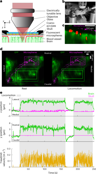
One month before window implantation, expression of GFP across brain cells22 was induced using retroorbital injection of 10 μl AAV (Addgene, cat. no. 37825-PHPeB, 1 × 1013 vector genomes (vg) ml−1) in 90 μl H2O (Supplementary Fig. 1b). We implanted a PoRTS window, with the additional step that fluorescent microspheres were applied to the surface of the skull (Fig. 1c and Supplementary Fig. 1a). In all mice, EMG electrodes were implanted in the abdominal muscles. Mice were then habituated to head fixation over several days before imaging.

Window and abdominal EMG surgery

Mice were anesthetized with isoflurane (5% induction, 2% maintenance) in oxygen throughout the surgical procedure. The scalp was shaved, and an incision was made from just rostral of the olfactory bulbs to the neck muscles, which was opened to expose the skull. A custom 1.65-mm thick titanium head bar was adhered to the skull using cyanoacrylate glue (Vibra-Tite, cat. no. 32402) and dental cement. To assist with head bar stabilization, two small self-tapping screws (J.I. Morris, cat. no. F000CE094) were inserted in the frontal bone without penetrating the subarachnoid space and were connected to the head bar with dental cement. A PoRTS window was then created over both hemispheres23. Windows typically spanned an area from lambda to rostral of bregma and were up to 0.5-cm wide, spanning across somatosensory and visual cortex. This allowed for maximum viewable brain surface. The skull was thinned and polished, and 1-μm diameter fluorescent microspheres (Invitrogen, cat. no. T7282) were spread across the surface of the thinned-skull areas (2 µl, 910,000 particles µl−1) and allowed to dry. The beads tended to form rings, similar to the patterns produced by drying coffee62. They were then covered with cyanoacrylate glue and a 0.1-mm-thick borosilicate glass piece (Electrode Microscopy Sciences, cat. no. 72198) cut to the size of the window. The position of bregma was marked with a fluorescent marker for positional reference, allowing for anatomical mapping across mice and a method of returning to imaging locations across several recording sessions.

To implant abdominal EMG electrodes, an incision 1 cm long was made in the skin below the rib cage to expose the oblique abdominal muscle. A small guide tube was then inserted into this incision and tunneled subcutaneously it reached the open scalp. Two coated stainless steel electrode wires (A-M Systems, cat. no. 790500) were inserted through the tube until the ends were exposed though both incisions, allowing the tube to be removed while the wires remained embedded under the skin. Two gold header pins (Mill-Max Manufacturing Corporation, cat. no. 0145-0-15-15-30-27-04-0) were adhered to the head bar with cyanoacrylate glue and the exposed wires between the header and neck incision were covered with silicone to prevent damage. Each wire exiting the abdominal incision was stripped of a section of coating and threaded through the muscle ~2 mm parallel from each other to allow for a bipolar abdominal EMG recording63. A biocompatible silicone adhesive (World Precision Instruments, KWIK-SIL) was used to cover the entry and exit of the muscle by the wires for implantation stability. The incision was then closed with a series of silk sutures (Fine Science Tools, cat. no. 18020-50) and Vetbond (3M, cat. no. 1469).

Multiplane imaging

To switch the focal plane rapidly between the brain and the skull, we integrated an electrically tunable lens (ETL) (Optotune, cat. no. EL-16-40-TC-VIS-5D-C) into the laser path (Extended Data Fig. 1a). The ETL was placed adjacent to and parallel with the back aperture of the microscope objective (Nikon, cat no. CFI75 LWD 16X W) to maximize axial range, avoid vignetting64 and remove gravitational effects on the fluid-filled lens that could alter focal plane depth or cause image distortion65. An ETL controller (Gardasoft, cat. no. TR-CL180) was used to control the liquid lens curvature. Preprogrammed steps in the curvature created rapid focal plane changes that were synchronized with image acquisition using transistor-to-transistor logic (TTL) pulses from the microscope. A microcontroller board (Arduino, Arduino Uno Rev3) was programmed to pass the first TTL pulse of every rapid stack to the ETL controller, which triggered a program that changed the lens curvature at predefined intervals (Extended Data Fig. 1b). The parameters of these steps were based on the frame rate, axial depth and number of images within the stack and were chosen to ensure the transitions of the lens’ curvature were done between the last raster scans of a frame and the beginning scans of the subsequent frame. The ability to trigger each rapid image stack independently using the microscope ensured consistent synchronization of the ETL and two-photon microscope even over long periods of data collection.

ETL calibration

We calibrated the ETL-induced changes in focal plane against those induced by translating the objective along the z axis (Extended Data Fig. 1). To generate a three-dimensional structure for calibration, strands of cotton were saturated with a solution of fluorescein isothiocyanate and placed in a 1.75-mm slide cavity (Carolina Biological Supply Company, cat. no. 632255). These cotton fibers were then suspended in optical adhesive (Norland Products, cat. no. NOA 133), covered with a glass cover slip, and cured with ultraviolet light (Extended Data Fig. 1d,e). At baseline, an ETL diopter input value of 0.23 was used as baseline as this generated a working distance closest to what would occur without an ETL. The objective was then stepped physically in the axial direction for 400 μm up and down in 5-μm steps, spanning 800 μm axially. The objective was then moved to the center of the stack and the diopter values were changed from −1.27 to 1.73 in 0.1 diopter steps while the objective was stationary, averaging 100 frames at each diopter value to obtain an image stack. The spatial cross-correlation between a single frame of the diopter stack and each frame of the objective movement stack were calculated to determine the change in focus location for each diopter value. This procedure was performed at three separate locations on the suspended fluorescein isothiocyanate cotton (Extended Data Fig. 1f). We performed calibrations of the magnitude across the usable range of ETL diopter values. Although the difference in micrometers per pixel scaling relative to the baseline focal values was large across extremes in ETL-induced axial focal plane shift, the typical range used for imaging the brains of mice (<100 μm) had a negligible effect (~0.01 µm per pixel) (Extended Data Fig. 1g).

To account for distortions of the image within the focal plane, we imaged a fine mesh copper grid (SPI Supplies, cat. no. 2145C-XA) (Supplementary Fig. 8). This square grid had 1,000 lines per inch (19-µm hole width, 6-µm bar width). These values were used to determine the micrometers per pixel in the center of each hole in both the x and y direction. This allowed us to generate two three-dimensional plots of x, y and micrometers per pixel points that were then fitted with a surface plot for distance calculations. The residuals of this fit were very small (nearly all <0.025 µm per pixel, Supplementary Fig. 8), showing that we can account for nearly all the distortion.

EMG, locomotion and respiration signals

EMG signals from oblique abdominal muscles were amplified and band pass-filtered between 300 Hz and 3 kHz (World Precision Instruments, cat. no. SYS-DAM80). Thermocouple (Omega Engineering, cat. no. 5SRTC-TT-K-20-36) signals were amplified and filtered between 2 Hz and 40 Hz (Dagan Corporation, cat. no. EX4-400 Quad Differential Amplifier)11. The treadmill velocity was obtained from a rotary encoder (US Digital, cat. no. E5-720-118-NE-S-H-D-B). Analog signals were captured at 10 kHz (Sutter Instrument, MScan).

The analog signal collected from the rotary encoder on the ball treadmill was smoothed with a Gaussian window (MATLAB function: gausswin, σ = 0.98 ms). Locomotion event onset was determined using a threshold between 0.05 and 0.1 m s−1 depending on mouse activity levels. EMG signal recorded from the oblique abdominal muscles from the mouse were filtered between 300 Hz and 3,000 Hz using a fifth-order Butterworth filter (MATLAB functions: butter, zp2sos, filtfilt) before squaring and smoothing (MATLAB function: gausswin, σ = 0.98 ms) the signal to convert voltage to power. Abdominal EMG contraction onset was determined using a threshold of ~100, or one order of magnitude increase from baseline power levels. The thermocouple signal was filtered between 2 Hz and 40 Hz using a fifth-order Butterworth filter (MATLAB functions: butter, zp2sos, filtfilt) and smoothed with a Gaussian kernel (MATLAB function: gausswin, σ = 0.98 ms).

Abdominal pressure application

A custom-made pneumatically inflatable belt (Supplementary Fig. 5a) was fabricated to directly apply pressure to the abdomen of mice. It consisted of three plastic bladders that were fully wrapped around the mouse abdomen. The belt was positioned between the rib cage and the hip bones of the mouse to ensure that pressure was applied only to the abdominal compartment between the diaphragm and pelvic floor. The belt was inflated with 7 psi of pressure to apply a steady squeeze for 2 s with 30 s of rest between squeezes to allow for a return to baseline (Supplementary Fig. 5b). The abdominal compression belt was oriented so that inflating portion was underneath the mouse so that no compression or tension was imparted to the spine longitudinally, as this could affect the results by pushing or pulling on the spine itself. Mice were observed with a behavioral video camera during imaging to check for potential compression-induced body positional changes and to monitor respiration.

Motion tracking

Brain and fluorescent skull bead frames were deinterleaved. Each frame was then processed with a two-dimensional spatial median filter (3 × 3, MATLAB function: medfilt2). Occasionally, a spatial Gaussian filter (ImageJ function: Gaussian Blur) and contrast alterations (ImageJ function: Brightness/Contrast) were also applied before the median filter if the signal to noise ratio of the images resulted in poor tracking analysis.

At least three locations within the image sequence were chosen as targets for tracking. These template targets were regions of high spatial contrast (for example cell bodies) selected manually and then averaged by pixel intensity across 100 frames during a period without brain motion to reduce noise for a robust matching template. Following the target template selection, a larger rectangular region of interest enclosing the template area was selected manually (MATLAB function: getpts) to restrict the search spatially (Fig. 1d and Extended Data Fig. 2d,f).

For tracking, a MATLAB object was created (MATLAB object: vision.TemplateMatcher). A three-step search method was typically deployed at this step to increase computational speed for long image sequences. The sum of absolute differences between overlapping pixel intensities was calculated between the target and search windows, and the minimum value was chosen as the target position within the image. To monitor motion tracking, a displacement vector was then calculated that showed the motion in pixels between the current and previous image frames which was used to translate each image into a stabilized video sequence (MATLAB function: imtranslate). For visualization, a stabilized image was displayed alongside the target box displacement in the original image (MATLAB object: vision.VideoPlayer) to aid in checking manually for tracking failure.

Once the displacement in pixels was calculated for each target in a frame, the matrix of these values was searched for unique rows (MATLAB function: unique) to determine the number of unique target locations within the image. We then calculated the corresponding real distance between each unique location and the midlines of the image. A line was drawn between the image midline and the pixel location of the target. Then the calibration surface plot that depicts the calibration value in micrometers per pixel at each pixel for both x and y directions was integrated across this line (Supplementary Fig. 8c, MATLAB function: trapz) to determine the distance in micrometers from the vertical and horizontal midline of the image. The real distance traveled between sequential frames was then calculated using these references by finding the difference of the target distances from the center of each frame. Performing the unique integrations first greatly increased the speed of processing the data. Motion was averaged across targets filtered with a Savitzky–Golay filter (MATLAB function: sgolayfilt) with an order of 3 and a frame length of 13 (at a nominal frame rate of 19.78 frames s−1)66. This filter was not applied to the position data in Fig. 2c before analyzing the frequency spectrum of the brain motion and its coherence with the thermocouple signal. The s.e.m. was calculated among the targets for each frame as well as the 90% probability intervals of the t-distribution (MATLAB function: tinv). The 90% confidence interval of the average object position in x and y was then calculated using the s.e.m. and the probability intervals for the three signals at each frame (Extended Data Fig. 4b). The displacement of the fluorescent microspheres on the skull was then subtracted from the displacement of the brain to obtain a measurement of the motion of the brain relative to the skull.

Motion direction quantification

We used principal component analysis to find the primary direction of brain motion. Displacement data was first centered around the mean, then the covariance matrix of the positional data was calculated (MATLAB function: cov). The eigenvectors of this covariance matrix were then calculated (MATLAB function: eig) to determine the direction of the calculated principal components. To determine the magnitude of the vector, we took the mean of the largest 20% of the displacements from the origin (MATLAB function: maxk) (Fig. 2a). We took the top 20% rather than the amplitude of the leading eigenvalue of the principal component because the eigenvalue is sensitive to locomotion amount. The amplitude of the leading principal component increases not just with the displacement amplitude, but also with the amount of time spent locomoting, so, for the same amount of locomotion-related displacement, the leading eigenvalue will be larger if there is more locomotion. To avoid this interpretation issue with the leading eigenvalue, we averaged the top 20% of the displacements, which proved robust to locomotion amount. This was done for each of the 316 recorded trials at 134 unique locations in 24 mice, where each trial is a continuous 10-min recording. For locations with several trials, motion vectors were averaged to produce a single vector (Figs. 2b and 5d and Extended Data Fig. 3b).

MicroCT and vascular segmentation

A C57BL/6 mouse (male, 27 weeks) and Swiss Webster mouse (female, 8 weeks) were anesthetized with 5% isoflurane in oxygen and perfused a radiopaque compound (MICROFIL, MV-120) to label the vasculature. The mice were then scanned with a microCT scanner (GE v|tome|x L300) at the PSU Center for Quantitative Imaging core (RRID: SCR_026734). The C57BL/6 mouse was imaged from the nose to the base of the tail, covering 99.36 mm separated into 8,280 slices with an isotropic pixel resolution of 12 μm. The Swiss Webster mouse was imaged from the diaphragm to the caudal edge of the hip bones, covering 49.73 mm separated into 4,144 slices with an isotropic pixel resolution of 12 μm (Supplementary Video 9). Images were collected using 75 kV and 180 μΑ with aluminum filters for best contrast of tissue densities. Segmentation was done with Slicer 3D52,67. Thresholding (3D Slicer function: thresholding) was first used to isolate the bone, and all voxels above a manually chosen intensity threshold were retained. Voxels that were preserved by the threshold tool but not required for the segmentation were removed within user-defined projected volumes (3D Slicer function: scissors). The result was a high-resolution reconstruction of the skull, ribs, vertebrae, hips and other small bones along the length of the mouse that retained their inner cavities. Segmentation of the vasculature surrounding the spine and skull was more difficult than isolating the bone because of the overlap in voxel intensity between the small vessels and the surrounding bone and tissues. The contrast agent also filled other organs (for example, liver) with a similar intensity, so a simple threshold could not be used for the vasculature. We separated the vessels by using a freeform drawing tool (3D Slicer function: draw) to encapsulate the desired segmentation area for a single slice in two dimensions while ignoring unwanted similar contrast tissues. This process was repeated along the spine with a spacing of ~100 to 200 slices between labeled transverse areas. Once enough transverse freeform slices were created, they were used to create a volume by connecting the outer edges of consecutive drawn areas (3D Slicer function: fill between slices). This served as a mask that required all segmentation tools used to focus only on the voxels within the defined volume and ignore all others. The initial segmentation of the vasculature was created using a flood filling tool (3D Slicer function: flood filling). This tool labels vessels that are clearly connected within and across slices to quickly segment large branches of the network. The masking volume was used here to ignore connections to vessels or organs outside of the wanted space. The flood fill tool did not detect some connecting vessels, particularly ones located near the inner and outer surfaces of the vertebrae. In these instances, we utilized a segmentation tool that finds areas within a slice that shares the same pixel intensity around the entire edge (3D Slicer function: level tracing) to fill these gaps. In comparison to the bone, the three-dimensional reconstruction of the vessels was not smooth as they were smaller and had much more voxel intensity overlap with surrounding tissues and spaces. Thus, the segmentation was processed with a series of slight dilation operations that were followed by a matched erosion (3D Slicer function: margin). This technique of growing and shrinking the object repeatedly smoothed the surface and linked gaps between vessels. A smoothing tool was then used for final polishing of the vasculature (3D Slicer function: smoothing).

Brain motion simulations

We aimed for our calculations to serve as a proof-of-concept of the ability of induced brain motion to drive fluid flow. Thus, we selected an extremely simple geometric representation of the mouse CNS (Fig. 6). The brain and spinal cord (in tan) are surrounded by communicating fluid-filled spaces (in cyan). These consist of a central spherical ventricle internal to the brain and the SAS on the outside of both brain and spinal cord. The SAS is connected to the ventricle by a straight central canal. In the center of the brain, above the ventricle, we placed a cavity meant to model the presence of the central sinus. In addition, we placed an outlet at the top of the skull to account for the fluid leakage out of the system through structures such as the cribriform plate. The dimensions for system’s geometry in the reference (initial) state are reported in Supplementary Table 1. As in Kedarasetti et al.16, both brain and fluid-filled spaces are modeled as poroelastic domains: each consists of a deformable solid elastic skeleton through which fluid can flow. The two domains, which can exchange fluid, differ in the values of their constitutive parameters, the latter being discontinuous across the interface that separates said domains. All constitutive and model parameters adopted in our simulations are listed in Supplementary Table 1.

The governing equations have been obtained using mixture-theory16,36,68 along with Hamilton’s principle37, following the variational approach demonstrated in ref. 38. Our formulation, detailed in ref. 39, differs from that in ref. 38 in that (1) each constituent herein is assumed to be incompressible in its pure form, and (2) the test functions for the fluid velocity across the brain/SAS interface are those consistent with choosing independent pore pressure and fluid velocity fields over the brain and SAS, respectively. Hence, the overall pore pressure and fluid velocity fields can be discontinuous across the brain/SAS interface. The Hamilton’s principle approach allowed us to obtain consistent relations both in the brain and SAS interiors as well as across the brain–SAS interface. In addition, this approach yielded a corresponding weak formulation for the purpose of numerical solutions using the finite element method (FEM)69.

By \(_}}(t)\) we denote the domain occupied by the cerebrum and spinal cord at time \(t\). Similarly, by \(_}}(t)\) we denote all fluid-filled domain, that is, the SAS in a strict sense along with the central canal and the ventricle, again at time \(t\). These domains are time dependent. We denote the interface between \(_}}(t)\) and \(_}}(t)\) by \(\Gamma ()\). The unit vector \(}\) is taken to be normal to \(\Gamma ()\) pointing from \(_}}(t)\) into \(_}}(t)\). To avoid a proliferation of symbols, we omit the notation ‘\((t)\)’ to indicate a domain at the initial time, that is, for \(t=0\), so that, for example, \(_}}=_}}\left(t\right)=0\). We denote the domain occupied by the system (that is, the mixture of the fluid and solid phases) by \(\Omega \left(t\right)\). This domain is the union of \(_}}(t)\) and \(_}}(t)\). As we have adopted a mixture theory framework, we posit the coexistence of a fluid phase and a solid phase at every point in \(\Omega (t)\). Although it is possible to conceive these phases to have different reference configurations, for convenience but without loss of generality, here we assume that the reference configurations of each phase coincide with \(\Omega\). Subscripts s and f denote quantities for the solid and fluid phases, respectively. In their pure forms, each phase is assumed incompressible with constant mass densities \(_}}^\) and \(_}}^\). Then, denoting the volume fractions by \(_}}\) and \(_}}\), for which we enforce the saturation condition \(_}}+_}}=1\), the mass densities of the phases in the mixture are \(_}}=__^\) and \(_}}=_}}_}}^\). The symbols \(}\), \(}\) and \(}\) (each with the appropriate subscript), denote the displacement, velocity and Cauchy stress fields, respectively. The quantity \(}}_}}=_}}(}}_}}-}}_}})\) is the filtration velocity. The pore pressure, denoted by \(p\), serves as a multiplier enforcing the balance of mass under the constraint that each pure phase is incompressible. To enforce the jump condition of the balance of mass across \(\Gamma ()\), we introduce a second multiplier, denoted ℘. The notation \([\kern-2pt[ a]\kern-2pt]\) indicates the jump of \(a\) across \(\Gamma ()\). We choose the solid’s displacement field so that \([\kern-2pt[ }}_}}]\kern-2pt] =\boldsymbol\) (that is, \(}}_}}\) is globally continuous). Formally, \(}}_}}\) and \(p\) need not be continuous across \(\Gamma ()\). Possible discontinuities in these fields have been the subject of extensive study in the literature (cf., for example, refs. 38,70,71) and there are various models to control their behavior (for example, often \(}}_}}\) and \(_}}\) are constrained to be continuous71). We select discontinuous functional spaces for \(p\) and \(}}_}}\) and we control their behavior by building an interface dissipation term in the Rayleigh pseudopotential in our application of Hamilton’s principle (similarly to ref. 38). This dissipation can be interpreted as a penalty term for the discontinuity of the filtration velocity. Before presenting the governing equations, we introduce the following two quantities: \(_}}=\left(1/2\right)_}}}}_}}\cdot }}_}}\) (kinetic energy of the fluid per unit volume of the current configuration) and \(d=_}}\left(}}_}}-}}_}}\right)\cdot }\), which the jump condition of the balance of mass requires to be continuous across \(\Gamma ()\).

The strong form of the governing equations, expressed in the system’s current configuration (Eulerian or spatial form; ref. 72) are as follows:

$$\nabla \cdot \left(}}_}}+}}_}}\right)=0\,}\,_}}(t)\cup _}}(t)$$

(1)

$$[\kern-2pt[ }}_}]\kern-2pt] \cdot }= 0\,}\,\Gamma ()$$

(2)

$$_}}}}_}}+_}}}}_}}-\nabla \cdot \left(}}_}}+}}_}}\right)=}\,}\,_}}(t)\cup _}}(t)$$

(3)

$$_}}}}_}}-\nabla \cdot }}_}}-}}_}}=}\,}\,_}}(t)\cup _}}(t)$$

(4)

$$[\kern-2pt[ _}}(}}_}}-}}_}})\otimes (}}_}}-}}_}})-}}_}}-}}_}}]\kern-2pt]} = }\,}\,\Gamma ()$$

(5)

$$_}}}-d\,}}_}}+_}}\wp }+}}_}}}-\frac_}}_[\kern-2pt[ }}_}]\kern-2pt] \right)}^=}\,}\,\Gamma ()$$

(6)

where \(}}_}}\) and \(}}_}}\) are material accelerations, the superscript ± refers to limits approaching each side of the interface, \(_\) is a viscosity like parameter (with dimensions of velocity per unit volume) characterizing the dissipative nature of the interface and where the terms \(}}_}}\), \(}}_}}\) and \(}}_}}\) are governed by the following constitutive relations

$$}}_}}=-_}}p}+2_}}}}_}}\frac_}}}}}_}}}}}_}}^}}+2_(}}_}}-}}_}})$$

(7)

$$}}_}}=-_}}p}+2_}}}}_}}+2_\left(}}_}}-}}_}}\right)$$

(8)

$$}}_}}=p\nabla _}}-\frac__}}^}_}}}\left(}}_}}-}}_}}\right)$$

(9)

where \(_}}\) is the strain energy of the solid phase per unit volume of its reference configuration, \(}}_}}=}+_}}}}_}}\) is the deformation gradient with \(_}}\) denoting the gradient relative to position in the solid’s reference configuration, \(}}_}}=}}_}}^}}}}_}}\), \(_\) is the Brinkmann dynamic viscosity, \(}}_}}=}}_}}\right)}_}}\), \(}}_}}=}}_}}\right)}_}}\), \(}\right)}_}}\) denoting the symmetric part of \(\nabla }\), \(_}}\) is the traditional dynamic viscosity of the fluid phase, \(_\) is the Darcy viscosity and \(_}}\) is the solid’s permeability. For \(_}}\) we choose a simple isochoric neo-Hookean model: \(\Psi =(_}}^/2)(^}:}}_}}-3)\), where \(J=\det }}_}}\) and \(_}}^\) is the elastic shear modulus of the pure solid phase. It is understood that the constitutive parameters in \(_}}(t)\) are different from those in \(_}}(t)\).

The details of the boundary conditions and of the finite element formulation are provided in the Supplementary Information. Here we limit ourselves to state that the problem is solved by using the motion of the solid as the underlying map of an otherwise Lagrangian–Eulerian formulation for which the reference configuration of the solid phase serves as the computational domain. The loading imposed on the system consists of a displacement over a portion of the dural sac of the spinal cord we denote as the squeeze zone, meant to simulate a squeezing pulse provided by the VVP. This displacement is controlled so that a prescribed nominal uniform squeezing pressure is applied to said zone. Flow resistance boundary conditions are enforced at the outlet at the top of the skull, and a resistance to deformation is also imposed on the walls of the central sinus.

Reporting summary

Further information on research design is available in the Nature Portfolio Reporting Summary linked to this article.