Mouse

All experiments were performed in compliance with protocols approved by the Institutional Animal Care and Use Committee at Cold Spring Harbor Laboratory (protocol number 22-6). Both female and male 2–14-month-old C57BL/6J mice were used in the experiments. Unless stated otherwise, animals were housed in an inverse light-to-dark cycle with constant temperature (20–22 °C) and humidity (54–59%), and had ad libitum access to water and food.

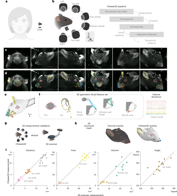
Video capture, synchronization and 3D calibration system

During the behavioral experiments, the mouse sits inside a custom 3D-printed tunnel and is head-fixed using a custom-made headpost (see CAD files at https://github.com/Hou-Lab-CSHL/cheese3d). The headpost is inserted into a metal rod and secured using a #2-56 thread, 1/4 inch screw tightened on a threaded hole on the side of the rod (see Extended Data Fig. 1). Six high-speed monochrome cameras (FLIR CM3-U3-13Y3M-CS 1/2” Chameleon 3) are used to record the video data at 100 fps. Based on their location relative to the face, the cameras are labeled left (L), right (R), top left (TL), top right (TR), top center (TC) and bottom center (BC) (see Fig. 1b and Supplementary Table 2). The camera location and orientation are selected such that each facial keypoint is in the focused view of at least two cameras (see Supplementary Table 1 for details). The sync LED, attached to the rod where the headpost is secured, is used as a fixed location on top of the mouse’s head, at the point of head fixation. The angle with respect to the sync LED is measured from a top-down view. The lateral cameras (L, R, TL, TR) are equipped with an 8 mm effective focal length (EFL) f/1.4 lens (MVL8M23, Thorlabs), and the center cameras (TC and BC) with a 12 mm EFL f/1.4 lens (MVL12M23, Thorlabs). Lenses are connected to the body of the camera through a C-to-CS-mount (03-618 Edmund Optics) and 3D-printed 1.1 mm (L, R, TL, TR cameras) or brass 2 mm spacer rings (TC, BC cameras) (03-633, Edmund Optics) for fine focal adjustment. The face is illuminated using two infrared lamps (CMVision IR30 WideAngle) with a piece of Kimwipe (Kimtech Science) covering the LED surface acting as a light diffuser to minimize glare. Most data were recorded using a Windows 10 desktop workstation with the following specifications: Intel Xeon Processor W-2265 (3.5GHz), 256 GB 8 × 32 GB DDR4 RAM, Nvidia RTX A6000 48GB, NVMe SSDs. For alternate setups (see Extended Data Fig. 3d), we used a commodity hardware laptop.

The six cameras were synchronized using Bonsai (v.2.8.1) and an Arduino Mega 2560 REV3, which sends a start signal to Bonsai through the serial port. Upon receiving the trigger signal, Bonsai begins recording frames from all cameras as well as associated metadata for each frame. This hardware signal ensures that different cameras are synchronized at acquisition time. To verify that the camera frames are synchronized post acquisition, a miniature infrared LED (SML-S13RTT86, Mouser Electronics) is positioned to appear in the field of view of all cameras. As a ground-truth synchronization signal, the LED is on for 10 ms every 10 ± 0.5 s.

Post hoc verification of camera synchronization is accomplished by detecting the frame of the rising edge of the LED signal in all views. Using the BC view as a reference, we linearly regress the rising edge times from another view onto the times from the reference view. A perfectly aligned pair of videos should regress onto the identity line, whereas a misaligned view will have a non-zero offset and non-identity slope. The non-zero offset is used as the frame shift to trim the non-reference video, and the slope is used to scale the effective frame rate to match the reference frame rate. This process is repeated systematically for all views and verified using the ground-truth synchronization LED signal.

Video-electrophysiology synchronization is conducted in a similar fashion, with the same synchronization LED signal split and connected to the electrophysiology hardware.

We calibrate camera views using a manufactured calibration board with a standard ChArUco template imprinted on its surface. A vectorized template for the ChArUco board was created using https://github.com/dogod621/OpenCVMarkerPrinter. The template used is for a 7 × 7 ChArUco board (4.5 mm marker length, 6 mm square side length, ArUco dictionary DICT_4 × 4_50). Before and after recording any experimental data, an experimenter held and rotated the ChArUco board in the focused view of all cameras for at least 1 min. These calibration videos were used in Anipose to calibrate the pipeline for triangulation using the default calibration settings.

Neural network keypoint detections and validations

We used video data from across all mice and experimental conditions (feeding experiments, awake recordings from the anesthesia experiment, recordings from the structure experiment, and so on) to train a single DLC model to track 2D keypoints. Three different DLC models were used throughout our analysis, except when noted otherwise. Differences between models are a result of dataset selection and training procedure (detailed below). For all models, random uniform sampling is used to separate 5% of the frames for testing, while the remaining 95% are used to train the model. Following the standard guidelines provided by DLC, we selected the built-in ResNet-50 model architecture and image augmentation pipeline for our training procedure. Model-specific descriptions are as follows:

For Figs. 1, 2, 3a–f, 4a–k, a total of 491 frames were selected using the k-means clustering algorithm for frame extraction provided by DLC, as well as manually (136 frames were manually taken from the feeding experiment). The model is trained for 1,030,000 iterations using a learning rate schedule of 0.005 for 10,000 iterations, 0.02 for 420,000 iterations, 0.002 for 300,000 iterations and 0.001 for 300,000 iterations. After training, the train set error was 2.16 pixels, and the test set error was 4.6 pixels.

For Fig. 5a–f, a total of 1,169 frames were selected using the k-means clustering algorithm for frame extraction provided by DLC. The model is trained for 1,630,000 iterations using a learning rate schedule of 0.005 for 10,000 iterations, 0.02 for 420,000 iterations, 0.002 for 300,000 iterations and 0.001 for 800,000 iterations. After training, the train set error was 3.3 pixels, and the test set error was 3.95 pixels.

For Figs. 3g–l, 4l–o, 5i–k, a total of 963 frames were selected using the k-means clustering algorithm for frame extraction provided by DLC, as well as manually (136 frames were manually taken from the feeding experiment). The model is trained for 4,700,000 iterations using a learning rate schedule of 0.005 for 100,000 iterations, 0.02 for 2,000,000 iterations, 0.002 for 1,000,000 iterations and 0.001 for 1,700,000 iterations. After training, the train set error was 1.92 pixels, and the test set error was 2.77 pixels.

Back-to-back 3D scanner and Cheese3D recordings in anesthetized mice were used to measure the spatial accuracy and resolution of keypoint detection (see Fig. 1 and Extended Data Fig. 2). Each mouse underwent intraperitoneal injection of ketamine (100 mg kg−1) and xylazine (10 mg kg−1) cocktail to induce anesthesia, and was scanned first on the 3D scanner (Einscan-SP, SHINING 3D) and then immediately on the Cheese3D setup.

To test the robustness of Cheese3D in detecting 3D keypoints, eight alternative setups were constructed by omitting either two or four cameras of the Cheese3D rig (Extended Data Fig. 3b,c for two examples), or varying camera positions and angles (Extended Data Fig. 3d). The four cameras composing the setup of Extended Data Fig. 3d were equipped with an 8 mm EFL f/1.4 lens (MVL8M23, Thorlabs), a C-to-CS-mount adaptor (03-618 Edmund Optics) and 3D-printed 1.1 mm spacer ring. Extended Data Fig. 3e compiles all setup variations, in which excluded cameras are marked with a dot. The design of these setups was based on an informed selection of cameras that could preserve the redundancy of as many keypoints as possible. For each setup, a new 2D model was trained from scratch, using only the labeled frames from the available views. Facial features were extracted and compared against the Cheese3D setup by computing the root mean square error, and the results are summarized in Extended Data Fig. 3e. Dotted squares indicate facial features that could not be calculated because of camera limitations (as some parts of the face were never seen) and were therefore discarded from analysis.

Triangulation and 3D tracking optimization

We use the trained DLC model to track keypoints in videos for each camera view separately for each experiment. No post-processing is applied to the tracked keypoints. Anipose is used to triangulate 2D keypoints from multiple cameras into a single 3D keypoint per frame using acquired calibration data (see ‘Video capture, synchronization and 3D calibration system’). Next, Anipose optimizes the 3D keypoint tracking for the full recording by reprojecting the 3D keypoints to 2D in each camera view and minimizing the mean squared error of the reprojected points. Concurrently, the frame-to-frame speed of the 3D keypoints is minimized to prevent spurious tracking errors. No post-processing or filtering is applied to the optimized 3D keypoints. To evaluate the performance of the tracking pipeline, we overlaid the optimized 3D keypoints reprojected onto each camera view, and an experimenter curated the accuracy and precision of the tracking results.

Comparison to an existing facial motion detection system

Recorded videos (640 × 512 pixels) were also tested with Facemap. A region of interest in each video was manually cropped using FFMPEG to match Facemap’s field of view. Although all views were given to Facemap, only the lateral cameras (R, L, TR, TL) resemble the canonical Facemap views. Keypoints were labeled using Cheese3D guidelines. Therefore, Facemap’s keypoints to track the right and left nostrils, nose bridge and paw were not implemented. Ears were not labeled, as Facemap’s base model does not include them. Facemap’s vibrissae keypoints, located at the base of three whiskers, were used to label Cheese3D whisker pad landmarks.

Visual inspection of the output tracking quality by several authors determined the need to fine-tune the Facemap model. For fine-tuning, two to ten frames per view and per experiment were selected using Facemap’s frame selection graphical user interface, resulting in a total of 166 frames. After the first iteration of refinement, some recordings still did not meet the team’s criteria for quality tracking (that is, assessed by visual inspection and jitter speed two orders of magnitude larger than Cheese3D’s), and additional fine-tuning was deemed necessary. For this second iteration, different fine-tuning branches of the same refined model were generated on a mouse basis using two frames per view. For the midline views (TC and BC) without any Facemap analog, an additional iteration of fine-tuning was sometimes required. We took the motionless periods (see ‘Analysis of kinematics during anesthesia’ for more information) to quantify 2D jitter. To make the outputs comparable, we reprojected the 3D output of Cheese3D into the six 2D views. We compared the average speed of the keypoints from each facial region (for example, eyes, nose) across views per mouse.

Anatomical-based interpretable feature selection

Features are selected and calculated in five tiers with increasing spatial dimension. First, 3D facial keypoints (see Fig. 1 and Extended Data Fig. 2) are selected based on the following criteria: they should be unambiguously and correctly pinpointed by at least three experimenters independently; for the purpose of 3D calibration, be in a focused view by at least two cameras; and reflect natural facial features and anatomy. Second, Euclidean distances between 3D keypoints within a localized facial region (for example, the left eye) are calculated. Third, areas are calculated for the sets of keypoints that form a closed polygon; these include the eye, ear and mouth areas. Fourth, the angle between the ear and snout is calculated as a measure for how forward-orienting the ears are with respect to the whole face. Fifth, the volumes of the nose bulge and whisker pad bulge are calculated to reflect anatomically relevant volumes5.

The areas of the eye and ear groups are calculated based on a flattened 2D ellipse. Each group consists of four points defining the major and minor axis endpoints of the ellipse. Given that all four points are not necessarily coplanar, we assume that the ellipse can be bent along the minor axis. To compute the area of this bent ellipse, we begin by defining the major axis (using the front and back of the eye or the base and tip of the ear). Next, we compute the midpoint of the major axis and calculate the Euclidean distance from this midpoint to each of the remaining two minor axis endpoints. The sum of these two distances defines the length of the minor axis after a potential bend has been flattened. Using the major and minor axis lengths, we compute the final ellipse area as the standard area of a 2D ellipse in Euclidean space. The area of the mouth can be computed as the standard area of a triangle in Euclidean space. The right and left upper lip points and one central lower lip point form the vertices of the triangle. The volume of the nose bulge is calculated as an irregular tetrahedron defined by the nose top, left and right pad top and the midpoint between the front of the eyes. We use the standard volume for an irregular tetrahedron in Euclidean space. The volume of the whisker pad bulge is calculated as an irregular pyramid defined by the nose bottom, left and right pad top, and left and right pad side points. We compute the convex hull defined by these points, then calculate the volume of the hull by dividing the hull into smaller tetrahedrons. The specific choice of tetrahedrons used is determined by the SciPy library (v.1.10.1). For a summary of the 17 facial features, see Supplementary Table 3.

Analysis of keypoint jitter

We quantified the tracking jitter of 3D keypoints and facial features using a 5 min video segment in which the experimenter identified no discernible movement (referred to as the ‘motionless period’). Next, we calculated the magnitude of the frame-to-frame speed of each keypoint during the selected periods that we refer to as the jitter speed of a keypoint. We use frame-to-frame speed as our metric for jitter so that we focus on short-time-scale noise in the tracking instead of slow-moving trends in the tracking that may occur over minutes or hours. To visualize the distribution of keypoint jitter speed in Fig. 2a, we compute a Gaussian kernel density estimate using the histplot function in the Seaborn plotting library (v.0.13.2). The bin size is set to 0.05 mm s−1, and the kernel density estimate bandwidth is set using the scotts_factor function in the SciPy library (v.1.10.1). We summarize the distribution of jitter speed during the motionless period by computing the average speed over the entire period per mouse in Fig. 2b.

To assess how the jitter speed of keypoints affects our anatomical features, we computed the absolute frame-to-frame speed of each feature during the selected periods, which we refer to as the jitter speed of an anatomical feature. We selected the 99.9th percentile of the anatomical jitter speed distribution per mouse as our motion threshold. Any movement with a frame-to-frame speed below this threshold will be considered noise. The motion threshold across mice is summarized in Extended Data Fig. 4.

Headpost design and surgery

The custom-designed stainless steel headpost for head fixation consists of a 6 × 4 × 1 mm rectangular base and a small 10 ×3 mm post that fits into the headpost holder. A groove was added on each lateral end of the base design to facilitate metabond adhesion during implant surgery. The headpost has a conical notch etched on the side to secure in the headpost holder with a screw fastener. The headpost holder is angled at 27.9∘, following observation of the natural head angle of the mouse eating to maximize comfort.

To implant the headpost, 2-month-old mice were anesthetized with isoflurane (SomnoFlo, Kent Scientific; 3–5% induction, 1–2% maintenance). Once anesthetic depth was achieved, mice were placed onto a stereotaxic apparatus where body temperature was maintained using a heating pad. After flattening the skull using skull landmarks, the base of the headpost is positioned above the medial-lateral midline and immediately anterior to lambda, and then secured using adhesive cement (Metabond, C&B). Following surgery, animals were administered buprenorphine (0.1 mg kg−1) and allowed to recover on a heating pad before returning to their home cages, in which they continued to recover for 1 week before being acclimated to sitting in a tunnel and head fixation for 1–2 weeks.

EEG surgery and data acquisition

One day before surgery, a biotelemetry unit (HD-X02, Data Sciences International) was thoroughly disinfected in CIDEX OPA solution (Advanced Sterilization Products). Surgery was performed as described above, with two stainless steel screws (00-96 × 1/16, EEG, IROX screw, Data Sciences International) inserted through craniotomy as cortical electrodes (screw 1: 1.5 mm anterior of bregma, 1.5 mm lateral of midline to the left; screw 2: 1.5 mm posterior of bregma, 3.5 mm lateral of midline, contralateral to screw 1. An incision was made to expose the upper trapezius muscles on the animal’s back to place the transmitter into the subcutaneous pocket. A pair of EEG leads was attached to the cortical screws and secured with a small amount of dental cement, and a pair of EMG leads was threaded through the upper trapezius muscles (one on each side of the midline) and held in place by 6-0 polyamide sutures. Tissue adhesive (3M Vetbond) was applied to the skull before attaching the headpost (described above). Post-surgery procedures were the same as described above, with at least 2 weeks recovery time before experiments.

Recording was conducted using a wireless recording system (Data Sciences International): transmitters communicated with PhysioTel receivers connected to PhysioTel Matrix MX2 acquisition interface. An Arduino MEGA generated a square signal that was synchronously sent to an infrared LED, visible in the Cheese3D camera system, and the PhysioTel Signal Interface, connected to the MX2 acquisition interface. The acquisition interface communicates with the EEG recording computer running Ponemah 6.5. All hardware devices are configured within Ponemah to record EEG, EMG and LED synchronizing signal at 1 kHz and body temperature at 1 Hz. After the experiment, data were exported to CSV format using NeuroScore 3.3.1 - Build 9317 (Data Sciences International).

In vivo electrophysiology recording, electrical stimulation surgery and data acquisition

Surgery was conducted as described above. A craniotomy was performed (anterior to bregma 1.5 mm, lateral 1.0 mm) to insert a grounding pin (male connector pin, A-M systems) at a 45° angle, with the tip of the pin pointing in the rostral direction. The skull was sealed with a tissue adhesive (3M Vetbond) before the headgear implant was attached and further secured with dental cement (C&B metabond, Parkell). The rest of the exposed skull was covered with additional dental cement to further secure the headgear in place. Post-surgery procedures were the same as described above, with at least 1 week recovery time before experimental water deprivation to aid acclimation (1–3 weeks) to awake head fixation.

Following acclimation, a 1 mm diameter brainstem cranial window was made above (posterior to lambda 1.8 mm, lateral 1.25 mm). Head-fixed mice were then stimulated under ketamine and xylazine anesthesia for three to five sessions (‘stimulation sessions’), followed by two awake acute recording sessions (‘recording sessions’). The camera configuration differs slightly from other datasets: the lateral and top center cameras (L, R, TL, TR, TC) are equipped with an 8 mm EFL f/1.4 lens (MVL8M23, Thorlabs), and the bottom center camera (BC) is equipped with a 12 mm EFL f/1.4 lens (MVL12M23, Thorlabs). In the first stimulation session, multiple brainstem locations were probed with a stimulation grid search. In subsequent stimulation sessions, a 32-channel four-shank silicon probe (A4 × 8-5 mm-100-200-177, NeuroNexus Technologies) was inserted at the mapped locations from the first session. Single electrical pulses (2 ms pulse duration, biphasic) were delivered to either the entire probe or specific divisions of individual shanks by Allego software (NeuroNexus Technologies) every 2–5 s. During the recording sessions, a 32-channel single-shank silicon probe with 46–54 kΩ impedance (H7b or H8b, Cambridge NeuroTech) was inserted into the brain region mapped during the previous stim sessions. The probe was coated with lipophilic dyes DiI or DiO (10% w/v) to reveal the probe track post hoc. Recordings began at least 15 min after probe insertion to ensure recording stability. Voltage signals were amplified using an RHD2132 amplifier (Intan Technologies) and acquired at 30 kHz with a NeuroNexus XDAQ ONE system. After the recording, single electrical pulses (0.5–2 μA) were delivered to all sites on the probe to induce facial movements to verify probe placement location.

Initial spike sorting was performed using Kilosort 2.5 with default parameters, followed by manual curation in Phy. Clusters with inter-spike interval violations, low signal-to-noise ratios or low stability through the recording session were excluded from single-unit analyses.

Analysis of kinematics during anesthesia

For the anesthesia experiments (see Fig. 3), the awake spontaneous movements of the mice were recorded in Cheese3D for 5 min, followed by intraperitoneal injection of a ketamine (100 mg kg−1) and xylazine (10 mg kg−1) cocktail to induce anesthesia, before returning to Cheese3D to record facial movement during and recovery from anesthesia. Temperature was maintained on a heating pad, and the exact time of injection was recorded. For the anesthesia re-dosing experiments, mice received either half of the original dosage of ketamine + xylazine or the equivalent volume in saline as a control. Around the 30 min mark from the first injection, the rig door was opened, and the mouse received the re-dosing injection while remaining head-fixed. The data points that were recorded 100 s before and after the second injection were excluded from further analysis. The experimenter was blinded to the content of the second injection.

To measure the wakefulness of each mouse during anesthesia, we computed the magnitude of the frame-to-frame speed of each anatomical feature over the entire recording. We labeled each time point as movement if the frame-to-frame speed crosses the previously computed motion threshold, while time points during which the speed is below the threshold are labeled as no movement. Fig. 3a shows an example raster plot of time points labeled as movement for one mouse.

We analyzed the slow drift of the anatomical and EEG features during anesthesia using a moving average of each feature during the entire recording period. The moving average is computed using a 10 s (facial features) or 40 s (EEG features) wide sliding window average. Fig. 3d shows exemplar filtered features for one mouse over the entire recording period. We visualized the filtered features across all mice and selected three representative features across three facial regions: left ear angle, left eye height and nose bulge. We trained a model across mice to predict time since injection using the selected features during anesthesia. Our model input consists of quadratic terms of the feature at the current time point and initial time point (quadratic terms computed using Scikit Learn’s (v.1.7.2) PolynomialFeatures class) as well as a constant bias. We performed a linear regression from our quadratic input terms to the current time since injection using the Lasso class from Scikit Learn (v.1.7.2), in which we used leave-one-out cross-validation and grid search (over 100 values from 0.1 to 100) to find the optimal regularization coefficient. A separate model was trained for features from the facial regions and the EEG frequency band powers. From a total of 12 sessions (across n = 3 mice), we held out three random sessions for testing and used nine for training, repeating this procedure 220 times. We assessed the performance of each model by predicting the time since injection for each test session. A moving-average-filtered (using the same filter as Fig. 3c,d) prediction for a single mouse and exemplar feature set is shown in Fig. 3e. We computed the average root mean squared error of the three sessions for each of the 220 runs in Fig. 3f.

For Fig. 3h,i and Extended Data Fig. 7, we trained models to predict each EEG frequency band power, using the three facial features of left ear angle, left eye height and nose bulge. All models are trained as a linear fit from facial features and past EEG frequency band power signal to current EEG frequency band power (and facial features) signal. To remain agnostic to the necessary features required for prediction, we trained several model classes where differences consist solely of variations on the features passed in and targets predicted out. These are illustrated in detail in Fig. 3h and Extended Data Fig. 7a, but we describe them in brief here. Input facial features consist of the three features during a sliding window of the past 1 min. Input autoregressive EEG features consist of the specific EEG frequency band power during a sliding window of the past 1 min. Additionally, for the time-latent model, the current time since injection is used as an exogenous input feature. The targets are either the current EEG frequency band power signal, current three facial features and the EEG frequency band power signal or the current time since injection. We trained four model classes:

Linear sliding window, which uses the sliding window facial features as input and current EEG frequency band power as target;

Linear autoregressive, which uses the sliding window facial features and autoregressive window of the EEG frequency band power as input and the current EEG frequency band power as target;

Linear vector autoregressive, which uses the sliding window facial features and autoregressive window of the EEG frequency band power as input and the current facial features and the EEG frequency band power as target;

Time-latent linear model, which trains two models: one uses the sliding window facial features as input and current time since injection as target, and the other uses the current time since injection and an autoregressive window of the EEG frequency band power as input and current EEG frequency band power as target.

For every model class, we train a different model for each mouse and EEG frequency band, using k-fold cross-validation across the recordings per mouse (using Scikit Learn’s model_selection.KFold class). We report results on the test folds only. In the case of the time-latent linear model, we train the two sub-models separately, then use the predicted time since injection from the first model as input to the second model, only for testing purposes. For visualization and measuring variance explained in Fig. 3h,i, we smooth the true and predicted EEG frequency band power using a moving average filter with a window of approximately 200 ms. We also report the same results on the unsmoothed data in Extended Data Fig. 7c,d.

For the anesthesia re-dosing experiment, to quantify the difference in facial features between the ketamine + xylazine and control saline solution, facial features were smoothed using a moving average filter with a window of 10 s and z-scored. We computed the cumulative running variance using a 6 s window. Then, we took the mean over a 5 min window and computed the difference 15 min before and after the second injection (see Fig. 3l).

Analysis of chewing kinematics

FED3 (ref. 59) was used to dispense chocolate-flavored 20 mg pellets (Dustless Precision Pellets, F05301, Bio-Serv) on demand during the feeding experiment (see Fig. 4). A funnel and tubing were placed underneath the FED3 spout to collect the dispensed pellet and deposit it on a translucent plastic spoon (Measuring Scoop S378, Parkell). The spoon was attached to a servo motor connected to a 3D-printed linear actuator to bring the pellet to the mouth, and then retracted to await the next pellet. Animals in the feeding experiments were gently food-restricted and acclimated for 2 days to eating from the spoon while head-fixed, to facilitate food consumption during the experiment. Each mouse was recorded eating 10 to 13 pellets in one session, and allocated 30 s per pellet. Dropped pellets were excluded from subsequent analysis. For Fig. 4l–o and Extended Data Fig. 9, mice received 50 pellets; dropped pellets were not excluded.

We distinguished the ingestion and mastication phases of chewing based on the shape of the lower envelope of the mouth area during the consumption of each pellet per mouse. An example lower envelope is shown in Fig. 4c. To compute the envelope, we invert the mouth area by negating it, then identifying the peaks of the negated signal using the find_peaks function in SciPy (v.1.10.1) with a window of 200 ms. The lower envelope is defined by linearly interpolating the calculated peaks, then median filtering the interpolated curve with a window of 1.49 s. We defined the transition time from ingestion to mastication as when the lower envelope drops sharply, as shown in Fig. 4c. To quantify the time when the envelope drops, we computed the cumulative area under the envelope during the consumption of each pellet. The cumulative area quickly increases during ingestion, then sharply transitions to a slower increase during mastication. The ‘knee’ in the cumulative area under the envelope was used to quantitatively define the transition time. We used the Kneedle algorithm (with the sensitivity parameter set to 1) to identify the knee point (transition time) for each pellet per mouse shown in Fig. 4d. The Python kneed (v.0.8.5) library was used as our Kneedle implementation.

In Fig. 4e,f, we compared the mouth area and nose bulge during the consumption of pellets by z-scoring each anatomical feature separately per pellet per mouse. For Fig. 4f, we plot the normalized mouth area and nose bulge against each other for an example mouse, in which each point constitutes a single frame. We color each point based on whether it occurs before or after the transition time for the corresponding pellet.

We defined the eye protrusion in Fig. 4h–k as the z-coordinate of the left eye back keypoint (we observed similar behavior for the right eye back). To quantify the degree of coordination between the mouth area and eye protrusion, we z-scored each feature per pellet per mouse. Next, we computed the cross-correlation between the normalized features per pellet per mouse separately for the ingestion and mastication phases. Fig. 4i shows the mean cross-correlation taken across pellets for a single mouse. We identified the peak cross-correlation by selecting the time point with the largest absolute cross-correlation per pellet per mouse, as shown in Fig. 4j,k.

In Fig. 4m–o and Extended Data Fig. 9, the ingestion-related mouth opening was determined as the first moment when the mouth area crossed over a 3 mm2 threshold within the first 2 s after spoon dispatch. When no value was found, usually when the pellet was not consumed, the largest possible value (that is, 2 s) was assigned. For Fig. 4m and Extended Data Fig. 9, a line was fitted to each mouse and session using the linregress function in SciPy (v.1.10.1). The mean slope resulting from the regressed lines per mouse was used to compute a two-sided Wilcoxon unpaired test, and the P value is reported in Fig. 4n. For Fig. 4o, mouse weight was calculated at the beginning of each session as a proportion of the original weight before food restriction.

Analysis of in vivo electrical stimulation and electrophysiological recording

Following data collection as described in ‘In vivo electrophysiology recording and electrical stimulation surgery and data acquisition’, video and ephys data were synchronized as described in ‘Video capture, synchronization, and 3D calibration system’. To obtain stimulus-triggered facial responses in Fig. 5b–f, a stimulus trigger signal aligning with the pulse duration was recorded on an analog channel of the electrophysiology data and used to drive an LED visible in the video data. For all but one of the sessions, the rising edge of the recorded trigger signal in the electrophysiological data was used as the time point for stimulus-triggered alignment. In one session, the analog channel was not available because of hardware failures, and the LED in the video was used instead.

Next, we computed the peak displacement of various facial features from their pre-stimulation baseline value. For 100 ms before the stimulation trigger, we measure the average value of a facial feature, then we define the peak displacement as the maximum (positive or negative) deviation away from the baseline average during a 100 ms period after the stimulation trigger. This is done on a trial-by-trial basis for each stimulation. In Fig. 5b (top right), we plotted the absolute value of the peak displacement for the eye height, taking the mean and standard deviation across trials of the same stimulation current amplitude.

We also evaluated our ability to distinguish stimulation-triggered movement from noise using the receiver operating characteristic (ROC) curve in Fig. 5b (bottom right). For a given stimulation current, taking a 100 ms period before stimulation as a ‘false positive’ response (noise) period and 100 ms after stimulation as a ‘true positive’ response (stimulation-triggered movement), we measure detected responses whenever the minimum ipsilateral eye height during the period was below a threshold. Sweeping the threshold from 10% below the minimum to 10% above the maximum eye height, we quantify the response rate during each period as the false positive rate and true positive rate for every threshold. From these data, we construct an ROC curve and measure the area under the curve (AUC) using NumPy’s trapz function. The ROC-AUC for each amplitude is shown in Fig. 5b.

In Fig. 5d, we show the absolute peak displacement of several facial features at 10 μA across all stimulation locations. We omitted some locations (appearing as white blank squares in the figure) when the peak displacement amplitude was below the jitter threshold for that feature, as defined in ‘Analysis of keypoint jitter’ and shown in Extended Data Fig. 5.

For in vivo electrophysiological recordings, spike trains were shuffled 1,000 times using a cyclic shuffling method, in which the entire spike train was shifted by a time between −60 s to −15 s or 15 s to 60 s60, with shifted spikes outside the time boundary wrapped to the start or the end of the time duration. To examine the correlation between neural activity and facial movements, actual or shuffled neural firing rates binned at 10 ms were cross-correlated with each facial feature. If the peak of the cross-correlation lies outside the 99.9% CI of the shuffled cross-correlation, and the corresponding lag is within −100 ms to 0 ms, the unit is considered statistically correlated with the facial feature (P < 0.001 as set by 1,000 shuffles). The significance of facial feature tuning was further assessed using 95% CIs of shuffled tuning curves and by manually verifying tuning specificity through facial video recordings overlaid with spike sounds.

To determine the predictability of neural activity from facial feature data, we trained a series of Poisson GLMs, also known as linear-nonlinear-Poisson models61. For all models, we binned spike trains into 10 ms spike count bins. On a per-recording basis, we trained a model for each facial feature and neural unit pair, in which a model receives a time window of facial features (corresponding to ±750 ms around the current time) to predict the current spike count. For each facial feature or unit pair, we train a model using tenfold cross-validation. To determine the folds, we take the full time range over a recording and partition the time into non-overlapping 10 s windows. A fold is a random sample of 10% of these windows (done using Scikit Learn’s model_selection.KFold class). Input feature windows that extend past the fold are discarded, and those time points are not used for training. Finally, the selected training data are used to fit a Poisson GLM with an intercept and L2 regularization with a strength of 1 × 10−8 (using Neural ModelS’s nemos.glm.PopulationGLM class). The solver used to perform fitting is a gradient descent method with a fixed step size of 1 × 10−2. For all figures, we report the prediction only on the test folds. Variance explained in Fig. 5j,k is computed as the mean squared difference between the predicted and true binned firing rate, smoothed by a 200 ms moving average filter. In addition to a cross-validated control, we also perform a negative control on randomized data. Specifically, we repeat the procedure described above 1,000 times, whereby each repetition uses chunk shuffled spike times (before binning) with 50 ms chunks.

Statistics and reproducibility

Required sample sizes were estimated based on previous publications and experience. The numbers of biological replicates, sessions and animals are reported in the figure legends. No data were excluded from analyses except for the following: for Fig. 1i, mouth area measurements were excluded owing to the lack of ground-truth measurements from the 3D scanner, as a result of the mouse’s orientation with respect to the projector. For Fig. 3j,l, ±100 s of data around the time of the second injection were excluded because the wireless receiver for the EEG was mounted on the rig door, and as such, opening the rig door for injection resulted in unreliable wireless communication during these periods. For Fig. 5g–k, clusters that did not pass spike sorting quality control (inter-spike interval violations, low signal-to-noise ratios or low stability through the recording session) were excluded from single-unit analyses.

Animals were randomly assigned to experimental groups where applicable for data presented in Fig. 3j,k,l; experimenters were blinded when necessary in Figs. 1, 3j–l and Extended Data Fig. 2. For the re-dosing experiment presented in Fig. 3j–l, the experimenters were blinded to the solution that was delivered to each group. The order of group assignment was randomly permuted for each animal. Specifically, bulk solutions for anesthetic and saline were prepared, and an external party blinded the injection solution independently for each session. The identities of all injections were not unblinded until all data analyses were complete, and the authors were unblinded only for producing the final figures. For comparison of Cheese3D against 3D scanner measurement in Fig. 1 and Extended Data Fig. 2, an experimenter obtained 3D positions for facial keypoints using Cheese3D, while an external party annotated 3D positions for the keypoints on the 3D scanner measurements following the same guidelines. The experimental and the third party obtained keypoints independently, blinded to each other’s selections, and the facial feature metrics were quantified and analyzed using automated pipelines applied identically across both sets of annotations, which were revealed to the experimenter when producing the final figures.

Reporting summary

Further information on research design is available in the Nature Portfolio Reporting Summary linked to this article.