The present study was performed in accordance with the recommendations laid out in the World Medical Association Declaration of Helsinki. Ethics approval was obtained from the Institutional Review Boards of the Beijing Children’s Hospital (IRB No. [2022]-E-207-Y) and the Institutional Review Boards of the Children’s Hospital of Chongqing Medical University (IRB No. 2023–488). Written consent was waived by the IRB as only retrospective data was used.

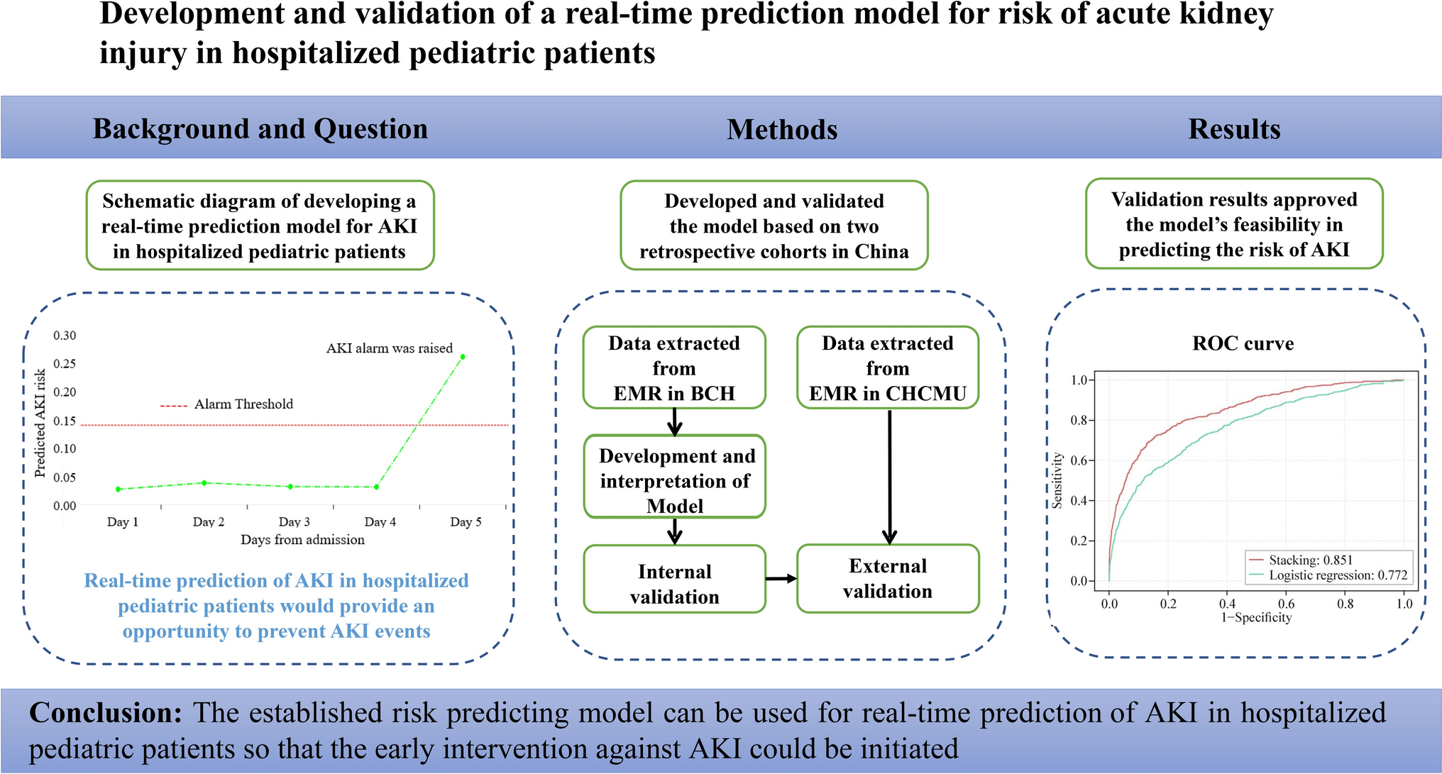
This study was performed using two retrospective cohorts from two pediatric hospitals in China. The Beijing cohort consisted of all patients hospitalized at Beijing Children’s Hospital, Capital Medical University from 2015 to 2020, with which we trained and performed an internal validation of the AKI prediction model. The Chongqing cohort consisted of all patients hospitalized at Children’s Hospital of Chongqing Medical University from Jan to June 2023, with which we performed an external validation of the AKI prediction model. Both Beijing Children’s Hospital and Children’s Hospital of Chongqing Medical University are tertiary care university teaching hospitals, located in North China and Southwest China respectively and are using different EMR systems. The same exclusion criteria were followed in both hospitals: (1) patients without at least two creatinine tests; (2) age under 28 days; (3) estimated glomerular filtration rate (eGFR) < 15 mL/minute/1.73 m2 or baseline creatinine > 4 × upper limit of normal (ULN) or diagnosed with chronic kidney disease (CKD) at admission, and (4) AKI developed within 24 hours of admission.

This manuscript is written following the Transparent Reporting of a Multivariable Prediction Model for Individual Prognosis or Diagnosis (TRIPOD) checklist [14].

First, a list of potential variables involved in model training was designed based on a review of prediction models of pediatric AKI and expertise in AKI occurrence and progress. Next, these variables were abstracted from EMR. The variables included demographics, comorbidities at admission, hospital procedures, drugs, laboratory testing data and vital signs. The variables with missing values exceeding 80% are excluded from statistical analysis. An advantage of the ensemble learning model is that redundant variables can be ignored, so a total of 75 variables were included in the model training to obtain a better predictive performance. A summary of these variables can be found in Supplementary Table 1. However, considering the ease of implementation of the model, we also performed feature selection using the genetic algorithm to obtain a simplified model. The results of the feature selection and the predictive performance of the simplified model are shown in Supplementary Table 2 and Supplementary Fig. 1.

Each predictor was classified as either a static or dynamic variable [15]. The static variables were defined as time-invariant during hospitalization and included demographics, comorbidities at admission and surgical procedures. Dynamic variables were values that were updated on a daily basis and included vital signs, laboratory testing values and drugs [16, 17]. All data in the observation window were used to predict AKI risk by merging dynamic variables in 24 hours with static variables.

The missing variables at baseline were imputed as median value [18, 19]. For missing values after admission, imputation was performed by the “last observation carried forward” method [20].

Numeric variables were scaled as follows:

$$}_=\frac-\upmu (\text)})}$$

Where μ(X) denotes the mean and σ(X) denotes the standard error of the feature X [21, 22].

The flow of data preprocessing as well as making real-time predictions is shown in Fig. 1. First, the updated dynamic variables for each patient are combined with the static variables to make a set of predictor variables (Fig. 1a). This way every patient in the data set was represented by a sequence of time steps (Fig. 1b) [23]. For each time step, the model would predict the occurrence of AKI in the next 24 hours (Fig. 1c). As a real-time prediction model, it will keep predicting AKI risk until actual diagnosis of AKI or discharge. Using the true test value of serum creatinine, we can determine whether the model is making correct predictions (Fig. 1d).

Diagram illustrating data preprocessing and the prediction window. A child developed AKI in the 6th day after admission was used as an example. A risk above 0.14 (corresponding to 50% precision) was the threshold above which AKI was predicted. AKI acute kidney injury, BUN blood urea nitrogen, PLT platelet, RBC red blood cell

AKI status was labeled according to the Kidney Disease Improving Global Outcomes (KDIGO) criterion [24]. Due to the relative sparsity of urine output data on the general hospital wards, urine output criteria for AKI were not considered. According to KDIGO guidelines an increase in serum creatinine of 0.3 mg/dL (26.5 μmol/L) within 48 hours or an increase in serum creatinine of 1.5 × the baseline creatinine level was identified as AKI. The same enzymatic method of serum creatinine measurement ensures diagnostic consistency between the two hospitals. Baseline creatinine was determined as the first creatinine measurement on admission. Onset time of AKI was labeled as the time of creatinine measurement on AKI diagnosis. The full-age-spectrum (FAS) equation was used to estimate glomerular filtration rate [25]. Two prediction windows were considered in this study, i.e., AKI within 24 hours or AKI within 24–48 hours.

Considering that the model is designed to predict the risk of AKI in real-time, it is evaluated daily for each patient during hospitalization. There are only 3.0% of time steps associated with a positive AKI label, indicating that the AKI prediction task is class-imbalanced.

To address class-imbalance, the technique of ensemble learning was employed [26, 27]. Ensemble learning combines several base models to improve learning efficiency. It has been shown that boosting models achieved good performance in AKI prediction models [28,29,30,31]. Thus, XGBoost, LightGBM and CatBoost were selected as base learners and were then combined using a stacking technique. Meanwhile, a logistic regression model was built for comparison with the stacking model.

To explore the best hyper-parameters of the stacking model, the particle swarm optimization (PSO) algorithm was used. This is an evolutionary algorithm designed by simulating the predatory behavior of a flock of birds [32]. Each base learner needs to be fine-tuned because they all have several hyperparameters. The PSO algorithm is expected to optimize the model more efficiently [33, 34]. An overview of the workflow for the modeling procedure is shown in Supplementary Fig. 2. The hyperparameter values are shown in Supplementary Table 3. The stacking model was fine-tuned within the derivation set through cross-validation to avoid overfitting.

The Beijing cohort was split into derivation and internal validation sets in such a way that information from a given patient was present only in one split. The derivation set was used to develop the proposed models and to tune the hyperparameters based on cross-validation methodology. To ensure independence between the derivation and internal validation set, we sampled based on patients instead of admission cases. In particular for patients with multiple admissions, all of their records were partitioned together either in the training or the test set.

The main performance indices used were: sensitivity (also known as recall), specificity, positive predictive value (PPV, also known as precision), negative predictive value (NPV), F1-score, the area under the receiver-operating curve (AUROC) and the area under the precision–recall curve (AUPR). Considering the feasibility of clinical prediction models in clinical practice, a cut-off value was chosen for the model to achieve at least 0.1 precision so that the number of false positives should ultimately not be a significant barrier to further implementation [23, 35]. A 10 × tenfold cross-validation was also conducted to obtain stable estimations of performance indices [36, 37].

The ensemble learning model cannot directly offer any explanations regarding the clinical meaning of features. We utilized the SHapley Additive exPlanation (SHAP) value, derived from game theory to determine the importance of features in our prediction model [38]. This is calculated by taking the average marginal contribution of all possible coalitions for a feature value. At the same time, the SHAP plots are figured to show the individual-level SHAP value and the importance of each variable in the prediction model.

Data preprocessing was conducted using SAS (version 9.4) and R (version 4.1.0). Descriptive statistical analyses were performed using SAS (version 9.4). The machine learning models were built and assessed using Python (version 3.10.4). Specifically, the categorical variables were summarized as counts and percentages (%), whereas real-time variables were described using median values and interquartile ranges (IQR). The differences between groups of categorical variables were compared using Chi-square or Fisher’s exact tests, and that of real-time variables were compared with the t-test or Wilcoxon rank sum test.