In this section, we apply the theoretical framework introduced earlier to real-world data. We first outline the modeling framework used to analyze the interactions among six opioid-related outcomes through a Bayesian spatial dynamic factor model. This approach allows us to capture the spatial and temporal dynamics of the opioid syndemic. We then present the results, highlighting the additional insights that spatially varying loadings provide compared to spatially constant loadings in understanding location differences in the syndemic.

We adopt the framework proposed by Hepler et al. (2019) to analyze the opioid syndemic in North Carolina (NC), focusing on the synergy between six opioid related outcomes: illicit opioid overdose deaths, emergency department visits related to drug overdose, treatment counts for opioid use disorder, patients receiving prescriptions for buprenorphine, newly diagnosed cases of acute and chronic HCV, and new diagnoses of HIV. For each outcome of interest, yearly, county-level counts are obtained for each of NC’s 100 counties from 2017 to 2021 from the NC Opioid and Substance Use Action Plan (OSUAP) Data Dashboard (Fliss et al. 2023), the 2021 North Carolina Hepatitis B/C Surveillance report (North Carolina HIV/STD/Hepatitis Surveillance Unit 2022), and the 2021 North Carolina HIV Surveillance Report (North Carolina HIV/STD/Hepatitis Surveillance Unit 2021). These data have also been used in (Murphy et al. 2025) to examine spatio-temporal patterns in opioid-related outcomes.

The six outcomes are jointly modeled using a Bayesian hierarchical spatial dynamic one-factor model. Specifically, for each location i, time j, and outcome k, we assume \(Y_^ \sim \text (E_^\lambda ^_),\) where \(\log (\lambda ^_) = \gamma ^_f_ + \varepsilon ^_\) and \(\varepsilon ^_ \overset\ N(0, \sigma ^2_k)\). Treatment counts between one and five are censored, which we account for in the model by adapting the censored generalized Poisson regression model of Famoye and Wang (2004). The expected counts, \(E_^\), are defined using the state average rate in 2017. Specifically, \(E_^ = P_r^\), where \(P_\) is the total population at location i in year j, and \(r^\) is the overall empirical state rate of outcome k in 2017. The factors, \(f_\), are modeled with a dynamic spatial factor model such that

$$\begin \begin f_|\pmb _&\sim N\left( \mu _1 + \sum _l \frac}}(f_ - \mu _1), \frac}\right) , \,\, \text j =1 \\ f_|\,}_ \}&\sim N\left( }_ + \sum _l \frac}}(f_ -}_), \frac} \right) , \,\, \text \,\, j=2,...,J. \end \end$$

In (13), \(}_ = \mu _ + \eta (f_ - \mu _)\) and \(\mu _j\) is an overall intercept for the factor in year j. That is, the factor assumes an intrinsic conditional auto-regressive (ICAR) structure to account for spatial autocorrelation and an autoregressive of order one structure to account for temporal autocorrelation. The \(w_\) elements, belong to the neighborhood matrix, which defines the spatial relationships between locations using an adjacency-based approach. That is, two locations are considered neighbors if they share at least one point. Accordingly, the (i, l) element equal to 1 if location i and l are neighbors and 0 otherwise. We let \(w_\) be the total of neighbors for location i.

For model identification, we assume \(\gamma _i^=1\) for all i, but we allow the loadings, \(\gamma _i^\) for \(k=2,...,6\), to vary spatially, specifying their structure using an ICAR model with mean one, to reflect the prior assumption that on average, the outcomes are all equally correlated to the latent factor. That is,

$$\begin \gamma ^_i|\gamma ^_ \sim N\left( 1 + \sum _l\frac}}(\gamma _-1), \frac}\right) . \end$$

(13)

Our model is fit in the Bayesian paradigm, and we assign weakly informative prior distributions for all remaining parameters. The variance components, \(\sigma ^2_k\), \(\tau ^2_f\), and \(\tau ^2_\) are assumed to have inverse gamma prior distributions with shape and scale parameters of 0.5, and the intercept parameters, \(\mu _j\), are assumed to have a uniform prior distributions on the real line. We use the nimble package (de Valpine et al. 2017) in R (R Core Team 2021) to implement a metropolis-within-gibbs markov chain monte carlo (MCMC) algorithm to sample from the posterior distribution of all model parameters. The MCMC algorithm is implemented for 1, 000, 000 iterations where the first 500, 000 iterations are discarded as burn-in, and subsequently, every 50th sample is retained. The choice of a longer burn-in and larger thinning interval was motivated by storage considerations. We established convergence by visually inspecting trace plots and by computing the Gelman-Rubin diagnostic. We conducted a sensitivity analysis on the precision parameters by testing alternative prior distributions. In addition to the original Gamma(0.5, 0.5) prior, we considered a Gamma(5, 2) prior. The standard deviation maps of the estimated latent factor showed no meaningful differences between prior specifications. With the model well-identified and relatively non-informative priors, the estimates remained consistent across these prior choices, indicating that our results are not sensitive to prior assumptions (see Figures SM26–SM30 in the supplementary material). The data and code for this analysis are available at https://github.com/evamurphy100/spatialloadings/tree/main.

In this subsection, we explore how the theoretical findings from the previous sections provide a more nuanced understanding of the opioid syndemic in North Carolina. We compare the interaction of six opioid-related outcomes under two scenarios: with spatially varying loadings and with spatially constant (non-varying) loadings.

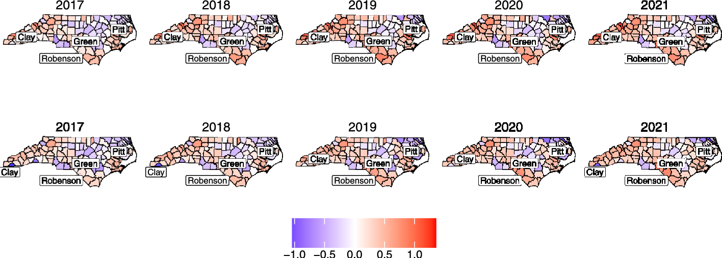
Maps of the estimated log relative risk for each outcome, shown in Figures SM8–SM13 in the supplementary material for the spatially varying loadings setup and Figures SM14–SM19 for the spatially constant loadings setup, closely resemble the empirical log relative risk maps in Figures SM20–SM25, reassuring the model’s goodness of fit to the data. Figure 1 and 2 compare the posterior means of the estimated latent factor with the two models: one with spatially constant loadings and the other with spatially varying loadings. To illustrate the spatial and temporal variation, we highlighted five counties: Clay County, with a population of 11, 231 people in 2021 as an example for low factor value; Robeson County, with a population of size 130, 625 people in 2021, as an example for high factor value; Pitt County, with a population of size 180, 742 in 2021; and Green County, with a population of size 21, 069 in 2021, as examples for medium factor values. At first glance, both factors appear very similar, showing a relatively subtle increase in the factor.

However, a closer examination of the time series graphs in Fig. 2 reveals prominent differences between the two factors. For example, in Robeson County, starting in 2019, the factor deviates more significantly from the median when loadings vary spatially, compared to when they are constant. In Clay County, the factor with spatially varying loadings shows an evident negative deviation from the median, with a substantial increase between 2018 and 2019 followed by a sharp decrease, in contrast to the factor with constant loadings. In Green County, the factor is significantly below the median when loadings vary spatially, as opposed to when they do not. These differences relate to our conclusion on the covariance structure of the outcome vector, \(}\). When the loadings are constant, it is assumed that the relationship between the factor (\(\pmb \)) and the outcomes (\(}\)) is the same in the spatial domain. This means that the spatial variation of \(}\) is mainly influenced by the spatial variation of \(\pmb \), forcing \(\pmb \) to account for most of the spatial variation in the outcomes across different counties, as previously mentioned. On the other hand, when the loadings vary spatially, they can adjust to how strongly \(\pmb \) influences \(}\) in the spatial domain. In this case, the variance of \(}\) depends not only on the variance of \(\pmb \) but also on the spatial variability of the loadings, allowing the model to account for regional differences. That is, this additional layer of spatial variation in the loadings can redistribute the observed variance, capturing localized effects. As a result, the trend in the factor may appear pronounced in some counties because spatially varying loadings allow the model to explain the variance of \(}\) differently in each location.

Posterior mean estimates of the latent factor from 2017 to 2021 with constant loadings (top row) and spatially varying loadings (bottom row). Zero indicates the state average in 2017

Posterior mean estimates of the latent factor over time with constant loadings (top) and spatially varying loadings (bottom). The grey region represents all counties that fall within the 2.5th quantile and 97.5th quantile of the rates. The state median and specific counties are highlighted using different line types

Table 1 shows the posterior mean estimates of the spatially constant loadings. Buprenorphine prescriptions receive the highest weight, with loadings values close to one, as expected, given their strong similarity to treatment counts. Death counts also have a loadings value closer to one, compared to the other outcomes: ED visits, HCV, and HIV, indicating a closer relationship between deaths, buprenorphine prescriptions, and treatment counts in the context of the opioid syndemic. This difference is reasonable, as ED visits include unintentional and undetermined overdoses with the potential for misuse, and HCV and HIV can be transmitted through methods unrelated to opioid use. We note that, under the assumption of spatially constant loadings, the way the factor influences the outcomes—and consequently, how the outcomes relate to the syndemic—remains the same throughout the entire spatial domain of North Carolina. This means that regardless of whether we are in Clay County, Robeson County, Pitt County, or Greene County, the outcomes contribute to the latent opioid syndemic in the same way.

With respect to spatially varying loadings, recall that we assume the mean of the loadings of each outcome k, \(k = 2, \ldots , 6\), is one. Under this assumption, a factor loading of one indicates that an outcome aligns with the latent factor to the same extent as the treatment outcome. The spatial maps of these raw loadings are shown in Figure SM1 of the supplementary material. However, interpreting the raw loadings in this format is challenging, as it requires comparison with the reference outcome, treatment. To facilitate interpretation, we scale the loadings and present the resulting spatial maps in Fig. 3. Scaling the spatially varying loadings involves dividing each loading by the sum of the six outcome loadings at the same location (Neeley et al. 2014). This allows for interpretation relative to \(1/6=0.167\), which serves as a baseline for equal contribution. Since the mean loading is assumed to be one, an outcome with a scaled loading of 0.167 at a given location contributes equally to the latent factor as the other outcomes at that location. Values above 0.167 indicate that the outcome has a stronger agreement with the latent factor, whereas values below 0.167 suggest that the outcome is less associated with the factor. For example, in the case of death counts, western counties such as Clay county have loading values below 0.167, whereas most central and eastern counties, including Robeson, Pitt, and Greene counties, have loadings above 0.167. This suggests that in western counties, death counts have a weaker correlation with the latent factor compared to other outcomes, whereas in central and eastern counties, they play a more prominent role. A similar pattern is observed for ED visits, with lower values in the western counties and higher values in the central-eastern counties. However, an interesting exception is Clay County, where ED visit loadings exceed 0.167, while in Pitt and Greene Counties, they are below this threshold. This suggests that in Clay County, ED visits are more strongly associated with the latent factor, whereas in Pitt and Greene Counties, they are less associated. Loadings for treatment and buprenorphine prescriptions are relatively consistent across North Carolina, with most values above 0.167, suggesting that these outcomes contribute more strongly to the factor. In contrast, loadings for HCV and HIV infections are generally below 0.167 across most counties, indicating that these outcomes are less associated with the latent factor and exhibit more independent behavior. This is expected as HCV and HIV can also be transmitted through non-opioid-related pathways so less variability is shared with the other opioid-related outcomes.

Scaled posterior mean estimates of the spatially varying loadings, computed by dividing each loading by the sum of all six loadings at each location. The color scale is centered at 1/6 (\(\approx 0.167\)), where values close to this indicate an equal contribution to the factor. Loadings greater or less than 0.167 represent areas of relatively higher or lower contributions, respectively. First row (left to right): death, treatment, ED visits. Second row (left to right): Buprenorphine, HCV, HIV

We provide maps of the posterior means of the outcome-specific errors, \(\varvec^\), \(k = 1, 2, \ldots , 6\), in Figures SM2–SM7 of the supplementary material. These plots suggest that the estimated errors tend to be smaller in the spatially varying loadings scenario compared to the spatially constant loadings scenario.

To further explore the role of spatially varying loadings, we assess the proportion of variance explained in each outcome. Specifically, we compute the ratio of the variance of the product of the loadings and factor to the total variance in each outcome. Fig. 4 displays these ratios, with red indicating values above 0.50 and blue representing values below 0.50. The figure suggests that ratios for the spatially constant loadings scenario are generally below 0.50, whereas ratios for the spatially varying loadings scenario are more often above 0.50. This indicates that spatially varying loadings account for a larger portion of the total variance compared to the spatially constant loadings. Allowing loadings to vary spatially helps capture more of the local variability in the outcome, whereas the spatially constant loadings provide a more averaged representation.

Proportion of variances explained by the product of loadings and factor relative to total variance for each outcome. Top row shows the ratios computed using spatially constant loadings, while the bottom row shows the ratios using spatially varying loadings. Red indicates values above 0.50, while blue represents values below 0.50