Our interest is in settings where one wants to evaluate the effect of a treatment on an endpoint that is a time T to an event of interest. In biomedical studies, one often cannot directly observe T, but can instead observe the time of last follow-up Y. This equals either a censoring time C if the last follow-up time occurs before T and equals T otherwise. That is, Y is the minimum of T and C: \(Y = \min \\). The binary variable \(\delta = I(T < C)\) equals 1 if the time to the event of interest was observed and equals 0 otherwise. The variable A indicates the treatment group membership with \(A = 0\) denoting membership in the control group of the study and \(A = 1\) denoting membership in the active treatment arm of the study. In addition to \((Y, \delta , A)\), we observe \(\textbf = (x_, \ldots , x_)\) which is a collection of p pre-treatment covariates. The data collected in such settings consists of n independent measurements of the form \(\, \delta _, A_, \textbf_ \}\), where \(i = 1, \ldots , n\).

To characterize HTE in settings with survival outcomes, one first needs to specify the treatment effect of interest. To define treatment effects, it is helpful to first define survival counterfactual (or potential) outcomes T(1) and T(0). Here, T(a) represents the survival time of an individual in treatment group a, and counterfactual survival outcomes T(a) and the survival outcome T are connected by the following

$$\begin T = AT(1) + (1 - A)T(0). \end$$

Frequently, a treatment effect of interest can be expressed as the expected difference in transformed counterfactual survival outcomes b(T(1)) and b(T(0)), for a monotone function of interest b(.). The expected difference \(E[b(T(1))] - E[b(T(0))]\) represents an average treatment effect because it does not condition on individual patient characteristics in any way.

Individualized treatment effects (ITE) – which are often referred to as conditional average treatment effects (CATEs) – represent average treatment effects among individuals that share a common covariate vector. Specifically, for a transformation function of interest b, the ITE at covariate vector \(\textbf\) is defined as

$$\begin E[ b(T(1)) \mid \textbf = \textbf] - E[b(T(0)) \mid \textbf=\textbf]. \end$$

Our main focus in this paper is on the ITE that contrasts expected survival on the log-time scale. This ITE function \(\theta (\textbf)\) is defined as

$$\begin \theta (\textbf) = \mathbb [\log (T(1)) \mid \textbf=\textbf] \;-\; \mathbb [\log (T(0)) \mid \textbf=\textbf]. \end$$

Under standard causal assumptions (e.g. consistency and no unmeasured confounding), this quantity corresponds to a contrast of the conditional expectation of the log of T with and without a treatment \(A\in }\) for a patient with covariates \(\textbf\). That is,

$$\begin \theta (\textbf) \;=\; \mathbb [\log (T)\mid A=1, \textbf=\textbf] \;-\; \mathbb [\log (T)\mid A=0, \textbf=\textbf], \end$$

(1)

In essence, \(\theta (\textbf)\) captures heterogeneity in treatment effects by quantifying how much longer (or shorter) an individual is expected to survive, on the log scale, with the treatment compared to without. We next describe two flexible modeling approaches for estimating \(\theta (\textbf)\) from censored survival data: AFT-BART and CSF estimators.

The AFT-BART method described in Henderson et al. (2020) focuses on utilizing flexible Bayesian machine learning tools to model individual-level survival distributions, and one can directly estimate the ITE function of interest by noting that any ITE is a feature of these individual-level survival distributions. With AFT-BART, individual-level survival distributions are built by using the Bayesian Additive Regression Trees (BART) framework (Chipman et al. 2010) to flexibly model covariate and treatment effects on the log failure-time scale. Specifically, the model posits that

$$\begin \log (T) \;=\; m(A,\textbf) \;+\; W, \end$$

(2)

where \(m(A,\textbf)\) is referred to as the regression function and \(W\) is a residual term with mean zero. Rather than assuming a linear (or otherwise simple) form for \(m\), AFT-BART uses a sum of regression trees:

$$\begin m(A,\textbf) \;=\; \sum _^ g(A,\textbf; \mathcal _j, \mathcal _j), \end$$

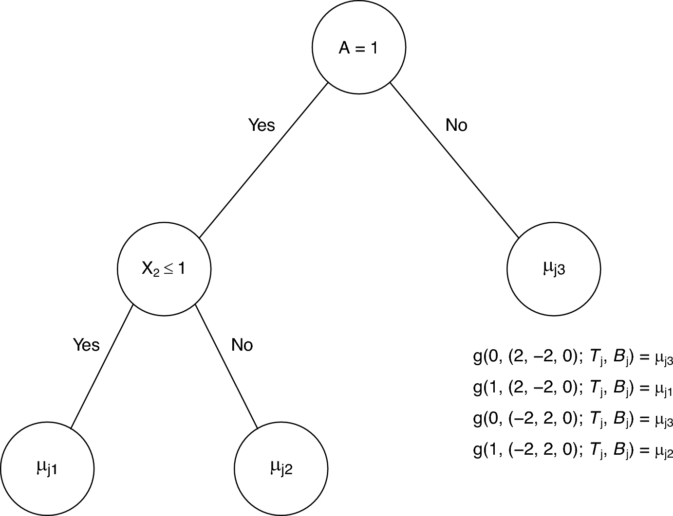
where each \(g(\cdot )\) is a function that returns the fitted value assigned by the decision tree \(\mathcal _j\) with leaf parameters \(\mathcal _j\) to the input treatment assignment A and covariate vector \(\textbf\). Figure 1 gives an example of a decision tree \(\mathcal _\) with leaf parameters \(\mathcal _\) and illustrates what value of \(g(A,\textbf; \mathcal _j, \mathcal _j)\) would return for several possible values of \((A, \textbf)\). The prior distribution on the regression function is fully specified through the priors on the collection of decision trees \(\mathcal _, \ldots , \mathcal _\) and associated leaf parameters \(\mathcal _, \ldots , \mathcal _\) with the tree priors usually chosen to generate short trees and shrinkage priors placed on the leaf parameters to better prevent overfitting. Further details on prior specification for \(\mathcal _\) and \(\mathcal _\) can be found in Chipman et al. (2010) and Henderson et al. (2020).

Under AFT model (2), the ITE function \(\theta (\textbf)\) for the difference in log-survival can be expressed as the difference in the regression function as:

$$\begin \theta (\textbf)= & E\ = \textbf \} - E\ = \textbf \} \\= & m(1, \textbf) - m(0, \textbf). \end$$

Illustration of a BART decision tree \(\mathcal _\) with three leaf nodes \(\mathcal _ = (\mu _, \mu _, \mu _)\). In this example, the covariate vector \(\textbf = (X_, X_, X_)\) has length three. Four choices of the treatment group variable A and covariate vector \(\textbf\) and the corresponding fitted value \(g(A, \textbf; \mathcal _, \mathcal _)\) are shown

Henderson et al. (2020) introduced two versions of AFT-BART: a fully nonparametric (AFT-BART-NP) and a semiparametric (AFT-BART-SP) specification. The main distinction between the NP and SP versions lies in how the residual distribution is modeled. The fully nonparametric version places a centered Dirichlet process mixture model prior on the error distribution, allowing maximum flexibility. In contrast, the semiparametric version assumes that the residual follows a Gaussian distribution with mean zero while still retaining the flexible BART prior for \(m(a,\textbf)\).

In this work, we primarily evaluate the semiparametric version, AFT-BART-SP, for two reasons. First, by incorporating some parametric structure on the residuals, AFT-BART-SP can improve efficiency and interpretability without sacrificing much flexibility in modeling covariate or treatment effects. Second, our aim is to compare performance with causal survival forest (CSF), which likewise adopts certain structural assumptions on survival outcomes. Using the SP variant thus provides a more directly comparable framework than the fully nonparametric specification.

Regarding censoring, the AFT-BART method assumes the right-censoring time C and the survival time T are independent. Under this assumption, a convenient approach for sampling from the posterior distribution of the regression function \(m(a, \textbf)\) and parameters of the residual distribution is to use a data augmentation strategy (Tanner and Wong 1987), where the unobserved survival times are treated as missing data. With this data augmentation strategy, which is commonly used in Bayesian approaches to the accelerated failure time model (e.g., Kuo and Mallick (1997)), one imputes these missing survival times in every iteration of the Gibbs sampler. To perform this imputation, one defines \(\tilde_\) to be the values of the unobserved survival times that have been right-censored, and under the assumption of independent right-censoring, one can show that the distribution of \(\log \tilde_\) given the observed data \((Y_, \delta _)\) and other model parameters is given by

$$\begin \log }_i \mid \log Y_i, \delta _ = 0, \;\sim \; \text \bigl (m(A_, \textbf_ ) + \tau _}, \sigma ^; \log Y_ \bigr ), \end$$

(3)

where the notation \(X \sim \text (\mu , \sigma ^; a)\) means that X has the same lower-truncated distribution as \(Z|Z > a\) where \(Z \sim \mathcal (\mu , \sigma ^)\). The term \(\tau _}\) in (3) is a cluster effect that is only relevant for the non–parametric version of AFT-BART, where the residual distribution is modeled with a centered Dirichlet process mixture model. In the semi–parametric version of AFT-BART, there are no cluster effects and \(\tau _}\) is always set equal to zero. After imputing the missing survival times via (3), one can sample the regression function and residual variance using standard sampling techniques in implementations of BART (Chipman et al. 2010).

Following (Cui et al. 2023), the CSF adapts the generalised random?forest machinery of (Athey and Imbens 2016) to right?censored outcomes. Using the notation of Section 2.1 and its identification assumptions, the estimand of interest is the conditional average treatment effect \(\theta (})=}[T_i(1)-T_i(0)\mid }_i=}]\). The forest consists of B honest survival trees. An honest tree is constructed by drawing a subsample without replacement and splitting it into a splitting subsample and an estimation subsample, so that covariate splits are chosen independently of the data later used for treatment–effect estimation and the resulting leaf estimates are conditionally unbiased (Wager and Athey 2018). Before tree construction, three nuisance functions are estimated: a propensity score \(}(})\) from a propensity forest, a censoring survival function \(}(t\mid })\) from a treatment–arm–stratified Kaplan–Meier estimator, and a baseline prognostic function \(}(})\) from an inverse–probability–of–censoring weighted regression forest whose responses are \(\delta _i Y_i/}(Y_i\mid }_i)\). Each observation is then mapped to the doubly robust pseudo–outcome

$$\begin }= \frac}(}_i)\}}}(}_i)\}(}_i)\}\,}(Y_i\mid }_i)} \bigl \}(}_i)\bigr \}, \end$$

(4)

which satisfies \(}[\hat_i\mid \textbf_i]=\theta (}_i)\). In the splitting subsample, each candidate split s is evaluated by the reduction in weighted mean–squared error of \(}\),

$$\begin Q(s)= \frac}_-}_\bigr )^2}}\!\bigl (}_-}_\bigr )}, \end$$

(5)

where \(\ell \) and r label the daughter nodes and the denominator uses the same inverse–probability weights; recursion stops when the estimation subsample of a node contains fewer than five observations. For a terminal node L the local effect is \(}=|L|^\sum _}\), and for a new covariate vector \(}\) the forest predictor is the adaptive–kernel average \(}(})=\sum _\alpha _n(L,})}\), where \(\alpha _n(L,})\) denotes the fraction of trees whose estimation leaf contains both \(}\) and the training units in L. Asymptotic variance is estimated by \(}_n(})=\sum _\alpha _n^2(L,})\,\widehat}(} i\in L)\), yielding Wald? type confidence intervals.