3.1 Notation

Consider a policy intervention that induces a distribution of drivers on the population receiving it. Our unit of analysis (the store) is the unit at which outcomes are measured and different driver levels could be defined, whereas distinct interventions are often delivered to groups of these units (e.g., regions). We index stores by \(i=1,...,n\), with each store in either the taxed (\(A_i=1\)) or control group (\(A_i=0\)). The intervention occurs between two time periods, \(t\in \\), and the binary time-varying tax status at time t is denoted by \(Z_=tA_i\). In each period, stores set the product price as \(\rho _\).

Analogously, units can be differentially exposed to drivers, which may induce tax effect heterogeneity. We define exposures to these drivers as follows: distance to the border \(B_i \in \mathbbm \), pass-through rate \(P_i = \rho _ - \rho _ \in \mathbbm \), and effective price competition \(h_(\varvec) \in \mathbbm \). Here, \(h_(\varvec)\) is a function of the prices of all study units at time t, \(\varvec\), similar to the exposure mapping function introduced by Aronow and Samii (2017). This function summarizes how stores are exposed to prices at neighboring stores, which we specify as the difference between \(\rho _\) and the minimum \(\rho _\) for j in the neighborhood of i, where neighborhoods are defined as the directly adjacent zip-codes of i. We separately define competition within Philadelphia (i.e., not including nearby, non-taxed stores) as \(h_(\varvec|A=1)\).

To distinguish between binary interventions and continuous drivers, we refer to the store’s level of exposure to the specific driver as the dose it receives. We observe outcomes such as volume sales, \(Y_\), in each period. Finally, we denote observed covariates as \(\mathbf \), which will be used to account for the effects of pre-intervention confounders and other drivers on outcome trends.

3.2 Causal estimands

In this section, we frame the hypothetical interventions from Sect. 2 as causal parameters, namely contrasts in potential outcomes. Depending on the research question, we define potential outcomes, \(Y_^)}\), according to a vector, \(\varvec\), of interventions and/or drivers subject to hypothetical intervention. Expectations in the following formulations are taken across units i, and we omit the unit subscript for simplicity. These estimands will be further demonstrated and interpreted in Sect. 4. For reference, acronyms and a short example are provided in Table 1.

3.2.1 Average treatment effect on the treated (ATT)

First, we consider the ATT, a common estimand in policy evaluations:

$$\begin ATT := E[Y_1^ - Y_1^|A=1]. \end$$

(1)

This estimand asks: “What would be the average difference in post-tax sales at Philadelphia stores had all stores been taxed compared to not taxed?” Here, \(\varvec=Z_\), since we only manipulate the tax status.

3.2.2 Average driver effect on the treated (ADT)

Second, we consider an effect curve, the ADT, as introduced in Hettinger et al. (2025). We define \(\mathbf \) and \(\varvec_}\) analogously to \(A_i\) and \(Z_\), but in the context of driver doses. Specifically, \(\mathbf \) represents the driver level assigned to a store, while \(\varvec_} = t\mathbf \) denotes the actual driver dose active at time t. Because we do not maniupulate \(\varvec_}\) under the control exposure in our hypothetical experiments in Sect. 2, we define \(\varvec=(Z_,\varvec_})\) when \(Z_=1\) and \(\varvec=Z_\) when \(Z_=0\). In our study, we will define drivers as uni-dimensional measures like distance to the border (\(\mathbf =B_i\)) and economic competition (\(\mathbf =h_(\varvec)\)), as well as a two-dimensional joint exposure of price change and economic competition (\(\mathbf =(P_i, h_(\varvec))\)). Then, the ADT is:

$$\begin ADT(\varvec) = E[Y_1^_}=\varvec)} - Y_1^ | A=1] \end$$

(2)

This estimand asks: “What would be the average difference in post-tax sales at Philadelphia stores were all stores taxed and exposed to the driver at level \(\varvec_1}=\varvec\) versus given the control exposure?”

3.2.3 Average treatment effect of a driver-unconfounded treatment on the treated (ADUTT)

Third, we consider the ADUTT:

$$\begin ADUTT(f_D) = \int \limits _\mathbbm E[Y_1^_}=\varvec)} - Y_1^ | A=1] df_D(\varvec) \end$$

(3)

This stochastic estimand asks: “What would be the average difference in post-tax sales at Philadelphia stores were all stores taxed but randomly assigned a driver level via \(f_D(\varvec)\) versus given the control exposure?” Without loss of generality, we assume \(f_D(\varvec) = p_D(\varvec|A=1)\) is the distribution of \(\textbf\) among the taxed region, to best align with the observed setting studied by the ATT. Thereby, the ADUTT can alternatively be interpreted as the average ADT over the realized distribution of doses.

3.2.4 Relative effect of driver assignment (REDA)

The ADUTT is often most relevant for comparisons to the ATT. Thus, we define the REDA to quantify how the ATT would relatively change if driver levels were independently assigned under the intervention:

$$\begin REDA = (ATT - ADUTT)/ATT \end$$

For example, a REDA of \(50\%\) implies that \(50\%\) of the ATT is explained by the non-randomness of driver dose assignment, whereas a REDA of \(-50\%\) implies that the intervention effect would be \(50\%\) higher under unconfounded driver dose assignment.

Table 1 Summary of key estimands with their corresponding interpretive questions3.2.5 Mathematical connection between the ATT and ADUTT

We can alternatively define the ATT under \(\varvec=(Z_,\varvec_})\) as:

$$\begin ATT=\int E[Y_1^_}=\varvec)} - Y_1^|A=1,\textbf] dp_(\textbf, \varvec|A=1) \end$$

This formulation of the ATT, which can be identified and estimated as the previous formulation, integrates over the joint distribution of confounders and driver doses, \(p_\), whereas the ADUTT integrates sequentially over the marginal distributions of X and D, i.e., \(p_X\) and \(p_D\):

$$\begin ADUTT=\int \limits _\mathbbm \int \limits _\mathbbm E[Y_1^_}=\varvec)} - Y_1^ | A=1, \textbf] dp_X(\varvec | A=1) dp_D(\varvec | A=1) \end$$

This distinction underscores the interpretation of the ADUTT as an effect under random, rather than confounded, driver dose assignment.

3.3 Identification assumptions

To identify these causal estimands, we require several (generally untestable) assumptions to map observable data to relevant counterfactuals.

3.3.1 Arrow of time (no anticipation)

We assume potential sales at time t are not influenced by future intervention status or driver dose. This condition would be violated, for instance, if consumers began altering their shopping habits before the tax was implemented. Previous studies have found limited evidence of this behavior in Philadelphia beverage tax data, suggesting that any violations of this assumption are likely minimal and unlikely to substantially bias our results (Hettinger et al. 2024; Roberto et al. 2019).

3.3.2 Modifed stable unit treatment value assumption (SUTVA)

We require a modified form of SUTVA, where potential outcomes depend on the population-level intervention status, \(\mathbf \), and driver levels, \(\varvec}_t}\) only through the individual unit’s intervention and driver status: \(Y_^, \varvec_t})} = Y_^, \varvec})}\). This assumption, which in part restricts how other units’ exposures influence a given unit’s outcome (i.e., interference), is often trivial in clinical trials by design but requires careful consideration in policy evaluations where spillovers may be more common. In our setting, when evaluating border proximity or price competition as the exposure, we assume that sales at store i in Philadelphia are unaffected by the exposure values (i.e., proximity or competition levels) of other Philadelphia stores, which appears reasonable in these cases. However, when considering price changes as the exposure, this assumption becomes less plausible, as sales at store i may be influenced by price changes at nearby stores. To address this, we represent the driver as bi-dimensional, \(\mathbf }=(P_i,h_(\varvec))\), in this hypothetical intervention. This allows us to adopt a more plausible form of interference, where consumer behavior is not strongly influenced by specific price changes at individual stores beyond a summary measure of neighborhood price competition (\(h_\)).

3.3.3 Consistency assumption

We assume that potential outcomes are equal to the observed outcomes equal the potential outcomes, \(Y_^, \varvec})} = Y_\), when \(Z_=z_\) and \(\varvec_}=\varvec}\).    

3.3.4 Positivity assumption

This assumption requires all units to have a non-zero probability of being assigned to each relevant intervention status and driver level. Essentially, it mandates sufficient overlap in covariates across the supports of intervention statuses and driver levels to balance confounders and extrapolate causal effects to the entire treated population.

3.3.5 Parallel trends assumptions

Finally, we require two forms of parallel trends:

1.

For the ATT, ADT, ADUTT, and REDA: A conditional counterfactual parallel trends assumption between treated and control units \(E[Y_^-Y_^ | A=1,\textbf] = E[Y_^-Y_^ | A=0,\textbf]\). This assumes that non-taxed stores are valid proxies for what would have happened to similar (by \(\textbf\)) taxed stores had no tax been implemented.

2.

For the ADT, ADUTT, and REDA: A conditional counterfactual parallel trends assumption among treated units between driver levels (Hettinger et al. 2025): \(E[Y_^)}-Y_^ | A=1,\mathbf }=\varvec,\textbf] = E[Y_^)}-Y_^ | A=1,\textbf] \text \varvec \in \mathbbm .\) This assumes that taxed stores exposed to driver level \(\varvec\) are valid proxies for what would have happened to similar (by \(\textbf\)) taxed stores had all Philadelphia stores received driver level \(\varvec\).

When these assumption do not hold, the estimated effects should be interpreted as associations between the intervention/driver and outcome that remain unexplained by observable factors.

3.4 Estimation approach

In this section, we summarize multiply-robust estimators for the ATT (Sant’Anna and Zhao 2020) and ADT (Hettinger et al. 2025) and introduce a new estimator for the ADUTT, whose efficient influence function has been previously derived (Hettinger et al. 2025). These semi-parametric approaches are essential to properly adjust for observed confounders without imposing the restrictive assumptions on effect heterogeneity inherent in TWFE frameworks (Abadie 2005; Sant’Anna and Zhao 2020).

3.4.1 Additional notation and key functions

We define the following conditional expectations:

Outcome trends among taxed stores given confounders and driver level: \(\mu _(\textbf, \textbf) = E[Y_1 - Y_0 | A=1, \textbf, \textbf]\)

Outcome trends among the non-taxed stores given confounders: \(\mu _(\textbf) = E[Y_1 - Y_0 | A=0, \textbf]\)

Additionally, we define the following probability functions:

Probability of being in a taxed region given confounders: \(\pi _A(\textbf) = P(A=1|\textbf)\)

Driver level density given confounders: \(\pi _D(\textbf, \textbf) = p(\textbf | A=1, \textbf)\)

Marginalized driver density: \(p(\textbf|A=1) = \int \limits _\mathbbm \pi _D(\textbf,\textbf) dp(\textbf|A=1)\)

These functions contribute to two composite functions based on the efficient influence functions for the ATT and ADUTT (Web Appendix A):

$$\begin \xi (\textbf, A, \textbf, Y_0, Y_1; \mu _, \pi _D)&= \frac(\textbf, \textbf)},\textbf)} P(\textbf|A=1) + \\&\hspace \int \limits _\mathbbm \mu _(\textbf, \textbf) dP(\textbf|A=1) \\ \tau (\textbf, A, Y_0, Y_1; \mu _, \pi _A)&= \frac)[(Y_1 - Y_0) - \mu _(\textbf)]}))} + \\&\hspace \frac\mu _(\textbf) \end$$

3.4.2 Estimation procedure 1.

Fit models for nuisance functions: \(\hat_\), \(\hat_\), \(\hat_A\), and \(\hat_D\). Section 3.5 provides guidance on confounder/exposure definitions, while Section  4.2 discusses implementation.

2.

Compute unit-specific contributions, \(\hat_i\) and \(\hat_i\), by plugging empirical data into \(\xi \) and \(\tau \) for all units. Integrals are approximated via sample means over treated units’ covariates for each driver level, \(\textbf\).

3.

For the \(ADT(\varvec)\), fit a non-parametric regression model (we recommend local linear kernel regression) as \(\widehat(\varvec) = \hat(\textbf)\), where \(\hat(\textbf)\) is obtained by fitting \(\hat\) as a function of \(\textbf\).

4.

Compute final estimates:

(a)

\(\widehat = \frac\sum \limits _^n [ \frac} (Y_-Y_) - \hat_i ]\)

(b)

\(\widehat(\varvec) = \hat(\varvec) - \frac\sum \limits _^n\hat_i\)

(c)

\(\widehat = \frac\sum \limits _^n[\hat_i - \hat ]\)

(d)

\(\widehat = \frac-\widehat}}\)

Table 2 summarizes robustness properties. Because \(\widehat\) depends on \(\tau \) but not \(\xi \), it only requires \(\hat_\) and \(\hat_A\) and is consistent if either are correctly specified. \(\widehat\), \(\widehat(D)\), and \(\widehat\) depend on both \(\tau \) and \(\xi \), thereby requiring both (i) either \(\hat_\) and \(\hat_A\) are correctly specified and (ii) \(\hat_\) or \(\hat_D\) are correctly specified.

Table 2 A summary of robustness properties of different estimators under different nuisance function specifications3.4.3 Inference

To conduct inference on these parameters, we use a weighted block bootstrapping approach to account for spatial correlation (Efron and Tibshirani 1993; Lahiri 1999). Implementation details are presented in Web Appendix B, while details on block specification are described further in Sect. 4.2. These bootstrapping approaches generally maintain robustness and can be readily adapted for different modeling approaches and spatial structures, unlike commonly used alternatives like sandwich estimators (Hettinger et al. 2025).

3.5 Accounting for other drivers and competition

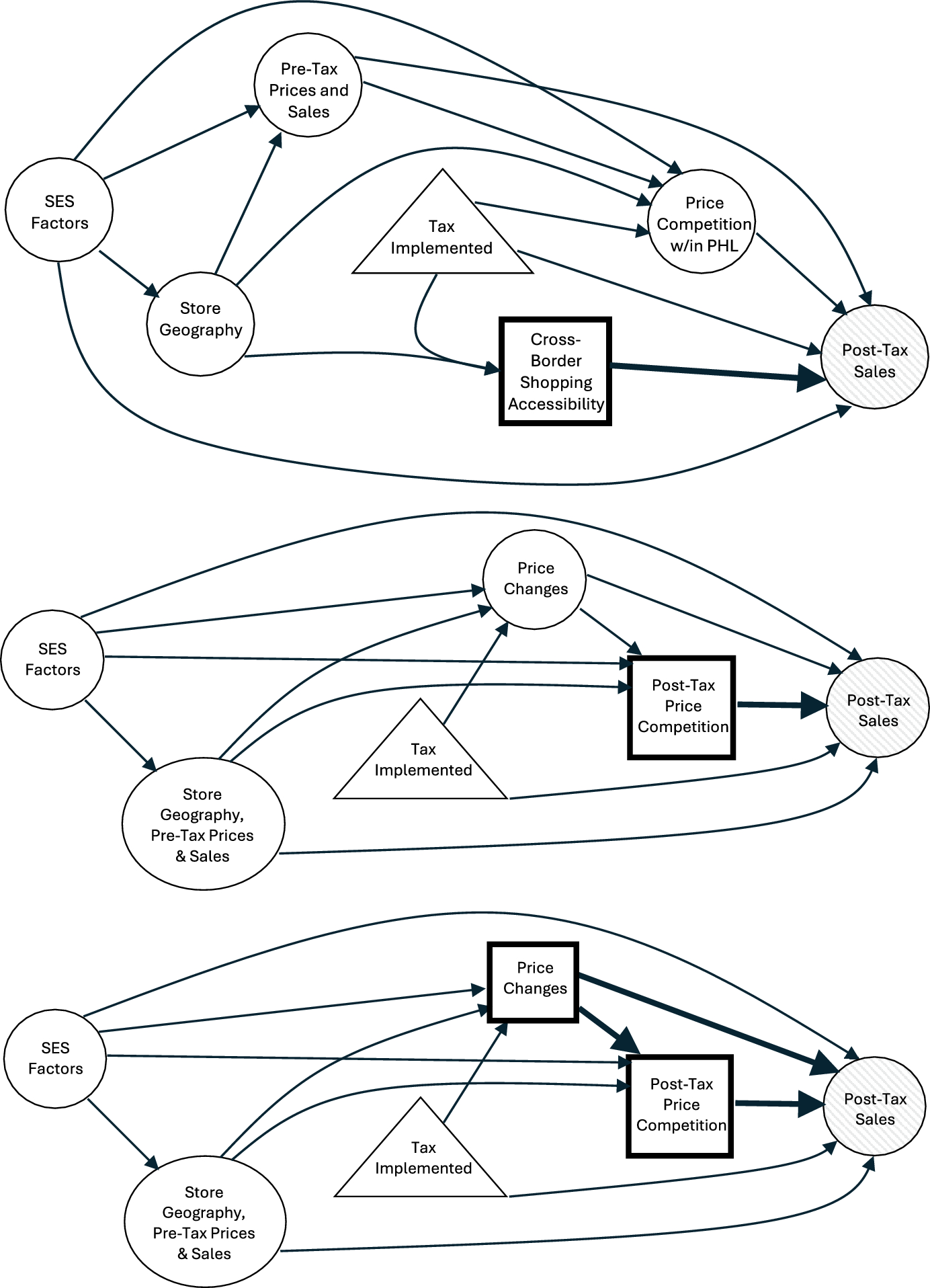
When estimating the impact of a specific driver, it is crucial to control for alternative causal pathways—such as those involving confounders like socioeconomic status, pre-tax prices, and pre-tax sales or other related drivers. When multiple drivers are causally linked or statistically associated, adjusting for non-target drivers as confounders is important, even if some emerge shortly after the intervention. However, caution is warranted when adjusting for variables downstream of, or interacting with, the driver of interest, as doing so may obscure its true effect by inadvertently blocking part of its causal mechanism.

To assess cross-border shopping effects via border proximity, we estimate the ADT while adjusting for pre-tax confounders (\(\mathbf \)) and price competition from other Philadelphia stores, \(h_(\varvec|A=1)\). However, we do not adjust for price changes, \(P_i\), or price competition from nearby non-taxed stores, as cross-border shopping effects largely operate through these price disparities.

To evaluate the impact of economic competition, we estimate the ADT while treating competition as the exposure of interest rather than a confounder. Here, we analyze a uni-dimensional driver (\(\mathbf }=h_(\varvec)\)) while adjusting for confounders (\(\mathbf \)). To determine whether consumers respond to observed, rather than presumed, economic competition, we also adjust for border proximity (\(B_i\)) and store-level price changes (\(P_i\)).

To evaluate how store-level price changes impact tax effectiveness, we estimate the ADUTT while ensuring price changes are not conflated with pre-tax factors influencing store pricing. Therefore, we adjust for confounders (\(\mathbf \)), border proximity (\(B_i\)), and pre-tax economic competition (\(h_(\mathbf ))\). Here, we define our driver as a joint measure of price changes and nearby price competition (\(\mathbf }=(P_i,h_(\mathbf ))\)), to emulate the hypothetical scenario where stores randomly adjust prices but price changes maintain their correlation with price competition.