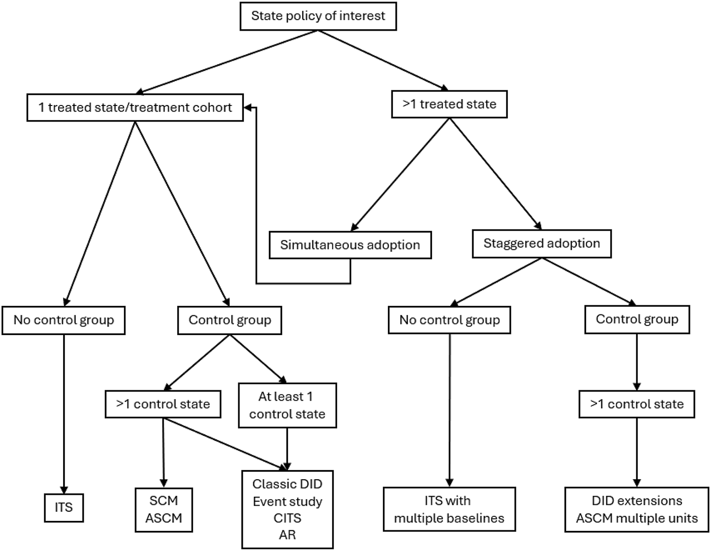
In the following sections, we detail analytic methods for state policy evaluations, with respect to the key design features highlighted above. Specifically, we differentiate between methods for the following settings: (1) single treated state/cohort, no comparison state(s), (2) multiple treatment cohorts (staggered adoption), no comparison state(s), (3) single treated state, multiple comparison states, (4) single treated state/cohort (simultaneous adoption), with comparison state(s), and (5) multiple treated states/cohorts (staggered adoption), with comparison state(s) (Fig. 1). Table 1 provides brief summaries of each method.

Fig. 1

Methods for policy evaluation. Figure depicts flow chart for identifying appropriate methods based on number of treatment states, timing of policy adoption, and presence and number of control states. Model assumptions, effect heterogeneity, data considerations, and relative model performance should be assessed and can be compared across models to inform selection of analytic approach. ITS interrupted time series, SCM synthetic control method, ASCM augmented synthetic control method, DID difference-in-differences, CITS comparative interrupted time series, AR autoregressive

Table 1 Common methods for policy evaluation4.1 Methods for a single treated state (or single treatment cohort), no comparison state(s)4.1.1 Interrupted time series (ITS)

In the interrupted time series (ITS) model, repeated measures over time (the “time series”) are used to assess changes in magnitude and trend of outcomes before and after a policy is enacted (the “interruption”). In its most basic form, the ITS model does not require a control group. The ITS model is expressed as:

$$g\left( }^}} \right)=+tim+polic+time\_since\_polic+}}+}$$

(1)

where \(\:g\left(.\right)\) denotes the generalized linear model (GLM) link function (e.g., linear), \(\:_\) denotes state fixed effects (in the case of multiple states in a single treatment cohort), and \(\:_\) denotes the error term. The measures in this model are \(\:time\), which measures time elapsed since the start of the study period, \(\:policy\), a time-varying indicator that denotes the policy is in effect at time \(\:t\), and \(\:time\_since\_policy,\:\)which measures time elapsed since the policy was implemented. In this model, the coefficients of interest are β2, which indicates the immediate change in outcome at the time of interruption (change in level), and β3, which indicates the change in outcomes over time following vs. before the interruption (change in slope).

Underlying causal assumption: The outcome in the treated state would have continued uninterrupted in both level and trend if not for the policy.

Key sensitivity analyses: placebo test of treatment timing (i.e., test pseudo-treatment time in the observed pre-period); placebo test of outcome (i.e., test policy effect on outcome not expected to be impacted); sensitivity to model specifications.

Model assumption(s): Ignorability, no anticipation, consistency.

Effect heterogeneity by time: Effect heterogeneity over time is captured in β3 which indicates the change in outcomes over time following policy adoption.

Effect heterogeneity by treatment cohort: Not applicable – single treatment state/cohort (effects assumed to be homogenous within treatment cohort).

Data consideration(s): Number of repeated measures, policy and outcome definition.

References: Berk (2022); Bernal et al. (2017); Ewusie et al. (2020); Kontopantelis et al. (2015)

4.2 Methods for multiple treatment cohorts (staggered adoption), no comparison state(s)4.2.1 ITS with multiple baselines

One extension of the basic ITS design is ITS with multiple baselines. In cases of staggered treatment adoption, there are different baseline periods for the different treatment cohorts. This staggered adoption allows for the estimation of effects in different states, with different baseline trends, and at different points in calendar time which help to account for temporal trends and other changes taking place at the time of the intervention. In ITS with multiple baselines, separate ITS models are fit for each treatment cohort and effects from all models can then be averaged.

Underlying causal assumption: The outcome in the treated states would have continued uninterrupted in both level and trend if not for the policy.

Key sensitivity analyses: placebo test of treatment timing; placebo test of outcome; approach to effect aggregation (e.g., simple average vs. weighted average); sensitivity to model specifications.

Model assumption(s): Ignorability, no anticipation, consistency, no spillover effects.

Effect heterogeneity by time: Effect heterogeneity over time is captured by the coefficient indicating the change in outcomes over time following policy adoption.

Effect heterogeneity by treatment cohort: Effect heterogeneity by treatment cohort can be assessed by comparing the separate results for each cohort; heterogeneity by treatment cohort is not formally tested.

Data consideration(s): Number of repeated measures, policy and outcome definition.

References: Biglan et al. (2000); Hawkins et al. (2007)

4.3 Methods for a single treated state, with more than one comparison state4.3.1 Classic synthetic control method (SCM)

The synthetic control approach is used to assess the impact of an intervention or policy change on a single state. This approach involves constructing a single “synthetic” control group (a weighted combination of control states) that matches the treated state as closely as possible on the outcome trends and potential confounders during the pre-policy period (Abadie et al. 2010). When creating the synthetic control group, states that are most similar to the policy state in the pre-policy period are “upweighted” (receive the largest weights) and states that are more dissimilar are “downweighted.” The effect estimate is then calculated as the difference between the treated group and the synthetic control in the post-policy period. Because SCM does not use an outcome model, p-values are calculated based on differences between observed values and permutation tests estimating placebo effects with control states. In contrast to the difference-in-differences designs (discussed below), SCM can explicitly account for time-varying confounders, as the weights match the treated and synthetic control group across the pre-policy period (Kreif et al. 2016).

Underlying causal assumption: The outcome trend and level in the synthetic control group in the post-period is what would have been observed in the treated state if not for the policy.

Key sensitivity analyses: placebo test of treatment timing; selection of control group.

Model assumption(s): Ignorability, positivity, no anticipation, consistency, no spillover effects.

Effect heterogeneity by time: Time-specific effects are automatically estimated in SCM programs.

Effect heterogeneity by treatment cohort: Not applicable – single treated state.

Data consideration(s): Number of repeated measures, policy and outcome definition.

References: Abadie (2021); Abadie et al. (2010); Abadie and Gardeazabal (2003); Abadie and L’Hour (2021).

4.3.2 Augmented synthetic control method (ASCM)

The augmented synthetic control method is an extension of the traditional SCM designed for settings in which traditional SCM’s weighting does not achieve satisfactory matching of the treated and control units in the pre-policy period (Ben-Michael et al. 2021). ASCM modifies the traditional SCM approach by (1) adding an outcome model to adjust for any remaining pre-treatment imbalances in outcomes or covariates between the treated state and the synthetic control and (2) allowing for negative weighting of control states, to provide better similarity in the pre-period. If traditional SCM achieves satisfactory weighting, results from traditional SCM and ASCM will be similar.

Underlying causal assumption: The outcome trend and level in the synthetic control group in the post-period is what would have been observed in the treated state if not for the policy.

Key sensitivity analyses: placebo test of treatment timing; selection of control group; sensitivity to model specifications.

Model assumption(s): Ignorability, positivity, no anticipation, consistency, no spillover effects.

Effect heterogeneity by time: Time-specific effects are automatically estimated in ASCM programs.

Effect heterogeneity by treatment cohort: Not applicable – single treated state.

Data consideration(s): Number of repeated measures, policy and outcome definition.

References: Ben-Michael et al. (2021)

4.4 Methods for single treated state or treatment cohort (simultaneous adoption), with comparison state(s)4.4.1 “Classic” (two-way fixed effect) difference-in-differences model (DID)

A common model in state policy evaluations is the classic two-way fixed effect difference-in-differences model (Dimick and Ryan 2014; Wing et al. 2018). DID has a long history in policy evaluation, harkening back to John Snow’s study of cholera in 1855 (Snow 1855). The DID estimate essentially subtracts the observed pre-policy to post-policy change in the comparison group from the observed pre-policy to post-policy change in the policy group, hence the name “difference-in-differences.” The classic DID specification is often implemented as a two-way fixed effects model that includes both state- and time-fixed effects expressed as:

$$g\left( }^}} \right)=+tr+polic+(trt) \times \right)_}+++}$$

(2)

where \(\:g\left(.\right)\) denotes the generalized linear model (GLM) link function (e.g., linear) and \(\:_\) denotes the error term. \(\:trt\) is a (time-invariant) indicator whether a given state is ever treated, \(\:policy\) is a time-varying indicator that denotes the policy is in effect at time \(\:t\), and \(\:\left(trt\right)\times\:\left(policy\right)\) term is the interaction of the two. β3, the coefficient of the interaction term, is the estimate of the treatment effect. State fixed effects, \(\:_\), quantify baseline differences in the outcome across states, and time fixed effects, \(\:_\), quantify national temporal trends. State fixed effects only account for time-invariant differences between states and time fixed effects only account for exogenous factors that affect both treated and untreated states equally.

Underlying causal assumption: If not for the policy, the treated state(s) would exhibit the same average change in the outcome from pre- to post-policy as was observed in the control state(s).

Key sensitivity analyses: selection of control group; sensitivity to model specifications.

Model assumption(s): Positivity, no anticipation, consistency, no spillover effects, parallel trends.

Effect heterogeneity by time: The event study/dynamic DID approach described below can be used to estimate time-specific treatment effects.

Effect heterogeneity by treatment cohort: Not applicable – single treated state or treatment cohort (effects assumed to be homogenous within treatment cohort).

Data consideration(s): Policy and outcome definition.

References: Abadie (2005); Baker et al. (2025); Bertrand et al. (2004); Chabé-Ferret (2017); Daw and Hatfield 2018a, 2018b; Ryan (2018); Ryan et al. (2015); Stuart et al. (2014); Zeldow and Hatfield (2021).

4.4.2 Event study/dynamic DID

The classic DID model generates a single point estimate for the policy effect, representing the average effect across the observed post-policy period. A notable and important extension to the classic DID model is the event study design, which has been employed in the economics literature since the 1930 s and allows for estimation of the time-varying effect of a policy (de Chaisemartin and D’Haultfœuille 2020). Essentially, an event time study defines time 0 as the time of policy implementation and examines time-specific treatment effects relative to a given time point (typically the time period immediately preceding policy adoption). The post-policy period is indexed by positive numbers (\(\:k=1,\dots\:,\:_\), where \(\:_\) represents the maximum number of time periods observed in the post-period) and accounted for in the model by “lagging indicators.” Inclusion of lagging indicators allows estimation of time-specific effect estimates in the post-policy period, thereby relaxing the classic DID assumption that the treatment effect is constant over time.

An event study model could also include “leading indicators” which span the pre-policy period (generally indexed by negative numbers \(\:k=-_,\dots\:,\:-1\), where \(\:_\) is the maximum number of time periods observed in the pre-period). Inclusion of these leading indicators requires extending the common trends assumption to also hold for the pre-policy period in addition to the post-policy period (Wing et al. 2018).

A full “DID event study” (or “dynamic DID”) includes the complete set of both leading and lagging indicators. The general form for a DID event time study is as follows:

$$\begin g\left( }^}} \right)= & +\mathop \sum \limits_}}^} \left( \right) \cdot polic}} \right)+\mathop \sum \limits_}^}} \left( \right) \cdot polic}} \right) \\ & +\beta }+}}++} \\ \end$$

(3)

where \(\:1(t=k)\) is an indicator that equals 1 if the observation’s event time indexed time is equal to \(\:k\) and 0 otherwise. The lagging indicators comprise the summation term indexed \(\:k=1,\dots\:,\:_\) and leading indicators comprise the summation term indexed \(\:_,\dots\:,\:-2)\). To avoid multicollinearity, one period is dropped (traditionally \(\:T=-1\)).

Underlying causal assumption: If not for the policy, the treated state(s) would exhibit the same change in the outcome trends from pre- to post-policy as was observed in the control state(s).

Key sensitivity analyses: selection of control group; sensitivity to model specifications.

Model assumption(s): Ignorability, positivity no anticipation, consistency, no spillover effects, parallel trends.

Effect heterogeneity by time: This model estimates time-specific treatment effects for each time point.

Effect heterogeneity by treatment cohort: Not applicable – single treated state or treatment cohort (effects assumed to be homogenous within treatment cohort).

Data consideration(s): Number of repeated measures, policy and outcome definition.

References: Freyaldenhoven et al. (2021); Miller (2023).

4.4.3 Comparative interrupted time series (CITS)

The comparative interrupted time series model is another extension of the basic ITS design which adds a comparison group. Conceptually the CITS design is similar to DID, though CITS requires more years of data. The basic CITS model extends the ITS model to include measures indicating treatment vs. control states and interactions of the treatment indicator with the time, policy, and time_since_policy variables:

$$\begin g\left( }^} } \right) = & \beta _ + \beta _ time_ + \beta _ policy_ + \beta _ time\_since\_policy_ \\ & + \beta _ treatment_ + \beta _ trtXtime_} + \beta _ trtXpolicy_} \\ & + \beta _ trtXtime\_since\_policy_ + \beta X_} + \rho _ + \varepsilon _} \\ \end$$

(4)

In this model, the coefficients of interest are β6, which indicates the difference in the immediate change in outcome at the time of interruption (change in level) between treatment and control states, and β7, which indicates the difference in change in outcomes over time following vs. before the interruption (change in slope) between treatment and control states. By comparing the trend of the outcome between the states that receive the policy change those that do not, the CITS model can estimate the magnitude and direction of the policy effect.

Underlying causal assumption: If not for the policy, the post-policy outcomes in the treated state(s) would have evolved in the same way as was observed in the control state(s).

Key sensitivity analyses: selection of control group; sensitivity to model specifications.

Model assumption(s): Positivity, no anticipation, consistency, no spillover effects.

Effect heterogeneity by time: Time-specific effects can be estimated using the CITS model.

Effect heterogeneity by treatment cohort: NA – the basic CITS model assumes simultaneous policy adoption (i.e., a single interruption). CITS models can be extended to account for multiple interruptions, though this is typically for multiple policy changes in a treated state or treatment group rather than for staggered policy adoption.

Data consideration(s): Number of repeated measures, policy and outcome definition.

References: Fry and Hatfield (2021); Lopez Bernal et al. (2018)

4.5 Methods for multiple treated States or treatment cohorts (staggered adoption), with comparison state(s)4.5.1 DID extensions: cohort-based DID extensions and Imputation-based DID extensions

Until fairly recently, the issue of staggered adoption – present in most state policy evaluations – was not given particular attention, as the classic DID model can (mathematically) handle this situation and provide a policy estimate. However, recent methodological work has highlighted that effect estimates from classic DID models may be biased in the presence of staggered adoption if policy effect heterogeneity exists (Borusyak et al. 2024; Callaway and Sant’Anna 2021; de Chaisemartin and D’Haultfœuille 2020; Goodman-Bacon 2021; Imai and Kim 2021; Sun and Abraham 2021). In the presence of staggered adoption, there are distinct “pre-policy” and “post-policy” periods with respect to each treated state that should be addressed. It becomes less clear which states should comprise the control group for a given treated state (e.g., only never-treated states? Or also not-yet-treated states?) and the models can inadvertently adjust for what are essentially “post-treatment” outcomes, which can lead to bias.

In particular, Goodman-Bacon (2021) showed that, in the context of staggered adoption, the classic DID is comprised of the weighted average of all possible comparisons of treated and control states. For example, assume that there are two groups of treated states, “early adopters” and “late adopters” in addition to a comparison group that never implements the policy of interest. There are now multiple possible comparisons: early adopters vs. untreated and late adopters vs. untreated, as well as the early adopters vs. late adopters (before the late adopter group implemented policy) and late adopters vs. early adopters (after the early adopter group implemented policy). Methodological work has characterized the latter two contrasts as “forbidden” contrasts that should be excluded as they include comparisons between groups that have already been treated, but initiated treatment at different times (Goodman-Bacon 2021). Furthermore, it has been shown that the classic DID estimator will only yield an unbiased estimate in the context of staggered adoption if the treatment effect is homogenous across states and across time (de Chaisemartin and D’Haultfœuille 2020). Systematic differences between states that adopt (vs. do not adopt) a policy and changes in policy implementation or enforcement over time that can impact the policy impacts (e.g., ramp up period to full implementation) make the assumptions of homogeneous treatment effects highly unlikely in most policy evaluations (Schuler et al. 2021). Multiple DID-based methods, such as those detailed below, have been recently developed specifically to handle staggered adoption and heterogeneous treatment effects.

One genre of DID extensions essentially creates a series of cohorts of states who implemented the policy at the same time, conducts a DID for each (having eliminated the issue of staggered adoption by re-anchoring time for each cohort), and then aggregates the cohort-specific estimates in various ways to summarize the overall policy effect. Having calculated these estimates for each group and time period, the group-time treatment effects are then aggregated to form an overall estimate of the treatment effect. Examples of cohort-based DID extensions include methods by Callaway and Sant’Anna (2021); de Chaisemartin and D’Haultfœuille (2020); Roth and Sant’Anna (2023); and Sun and Abraham (2021).

Another category of DID-based extensions can be termed imputation-based methods. For example, a method proposed by Borusyak et al. (2024) uses all untreated observations (i.e., all observations from “never treated” states + pre-policy observations from “not yet treated” states) to estimate a classic two-way fixed effect DID model. Using this untreated sub-sample estimates a “counterfactual” for each treated unit in the absence of treatment. Next, the treatment effect is calculated as the (population-weighted) average of the difference between the observed outcome and the predicted counterfactual, \(\:_^-}_^\). These approaches yield valid estimates when the parallel trend assumption holds for all groups and time periods and there is no anticipation effect.

Underlying causal assumption: If not for the policy, the treated state(s) would exhibit the same average change in the outcome from pre- to post-policy as was observed in the control state(s).

Key sensitivity analyses: selection of control group; sensitivity to model specifications.

Model assumption(s): Positivity, no anticipation, consistency, no spillover effects, parallel trends.

Effect heterogeneity by time: These cohort- and imputation-based approaches can easily be conducted in a way that estimates time-specific treatment effects.

Effect heterogeneity by treatment cohort: Somewhat by definition, the cohort-based analyses estimate cohort-specific treatment effects. Imputation-based DID extensions do not use treatment cohorts but individual DID models can be estimated for each treated state or treatment cohort.

Data consideration(s): Number of repeated measures, policy and outcome definition, policy treatment cohorts.

References: Overview of DID extensions: Roth et al. (2023); Wang et al. (2024); Cohort-based DID extensions: Callaway and Sant’Anna (2021); de Chaisemartin and D’Haultfœuille (2020); Roth and Sant’Anna (2023); Sun and Abraham (2021); Imputation-based DID extensions: Borusyak et al. (2024); Gardner (2022); Liu et al. (2024); Powell et al. (Under Review)

4.5.2 Debiased autoregressive (AR) models

Debiased autoregressive models are another class of methods recently highlighted as promising for policy evaluation (Antonelli et al. 2024). Standard autoregressive models include one or more lagged measures of the outcome variable (e.g., \(\:_^\)) as covariates. However, when estimating causal effects, incorporating lagged outcomes into models can lead to biased effect estimation when the lagged outcomes capture parts of the policy effect (Griffin et al. 2021; Schell et al. 2018). A recently proposed solution to this problem are so-called “debiased autoregressive models.” These remove effects of the policies from prior periods as a strategy to obtain unbiased causal effects while controlling for potential confounding from differences in prior outcome trends absent treatment across treated and comparison states. One parameterization of a debiased AR model with a single lagged value of the outcome expressed as \(\:_^\:\)is:

$$g\left( }^}} \right)=+(} - \gamma ~polic})+\gamma ~polic}+\beta }++}$$

(5)

Like the classic DID model, this model includes time fixed effects that capture temporal trends. However, the model also adjusts for state-specific variability using the debiased AR term (\( \left( \cdot \left( }^} - \gamma \:policy_} } \right)} \right) \) rather than state fixed effects. Notice that in a setting where states are only treated in the final time period, \(\:polic_\) is zero for all units, so that in this setting this becomes a standard AR model.

Underlying causal assumption: The policy is effectively randomized at every time point conditional on the covariates and the prior outcomes absent the policy.

Key sensitivity analyses: specification of lagged term(s); selection of control group; sensitivity to model specifications.

Model assumption(s): Ignorability (conditional on covariates and prior outcomes absent treatment), positivity, no anticipation, consistency, no spillover effects.

Effect heterogeneity by time: This model can utilize an event study/dynamic approach similar to DID to estimate time-specific treatment effects.

Effect heterogeneity by treatment cohort: This model can be used to estimate cohort-specific treatment effects by directly including both the main effects of cohorts as well as cohort interaction effects in the model.

Data consideration(s): Number of repeated measures, policy and outcome definition.

References: Antonelli et al. (2024); Schell et al. (2018)

4.5.3 ASCM extension for staggered adoption

The augmented synthetic control method can be extended for settings with staggered treatment adoption. In this approach, the synthetic control units are weighted to minimize a weighted average of pooled and unit-specific pre-treatment fits. This combination can range from 0, with separate synthetic control weights estimated for each treatment unit, to 1, a fully pooled synthetic control weighted to estimate the mean across all treated units; a partially pooled approach is recommended (Ben-Michael et al. 2022).

Underlying causal assumption: The outcome trend and level in the synthetic control group in the post-period is what would have been observed in the treatment cohorts if not for the policy.

Key sensitivity analyses: placebo test of treatment timing; selection of control group; sensitivity to model specifications.

Model assumption(s): Ignorability, no anticipation, consistency, no spillover effects.

Effect heterogeneity by time: Time-specific effects are automatically estimated in ASCM programs.

Effect heterogeneity by treatment cohort: The program used to implement this method can also estimate effects by treatment cohorts (a separate synthetic control is generated for each cohort).

Data consideration(s): Number of repeated measures, policy and outcome definition, policy treatment cohorts.

References: Ben-Michael et al. (