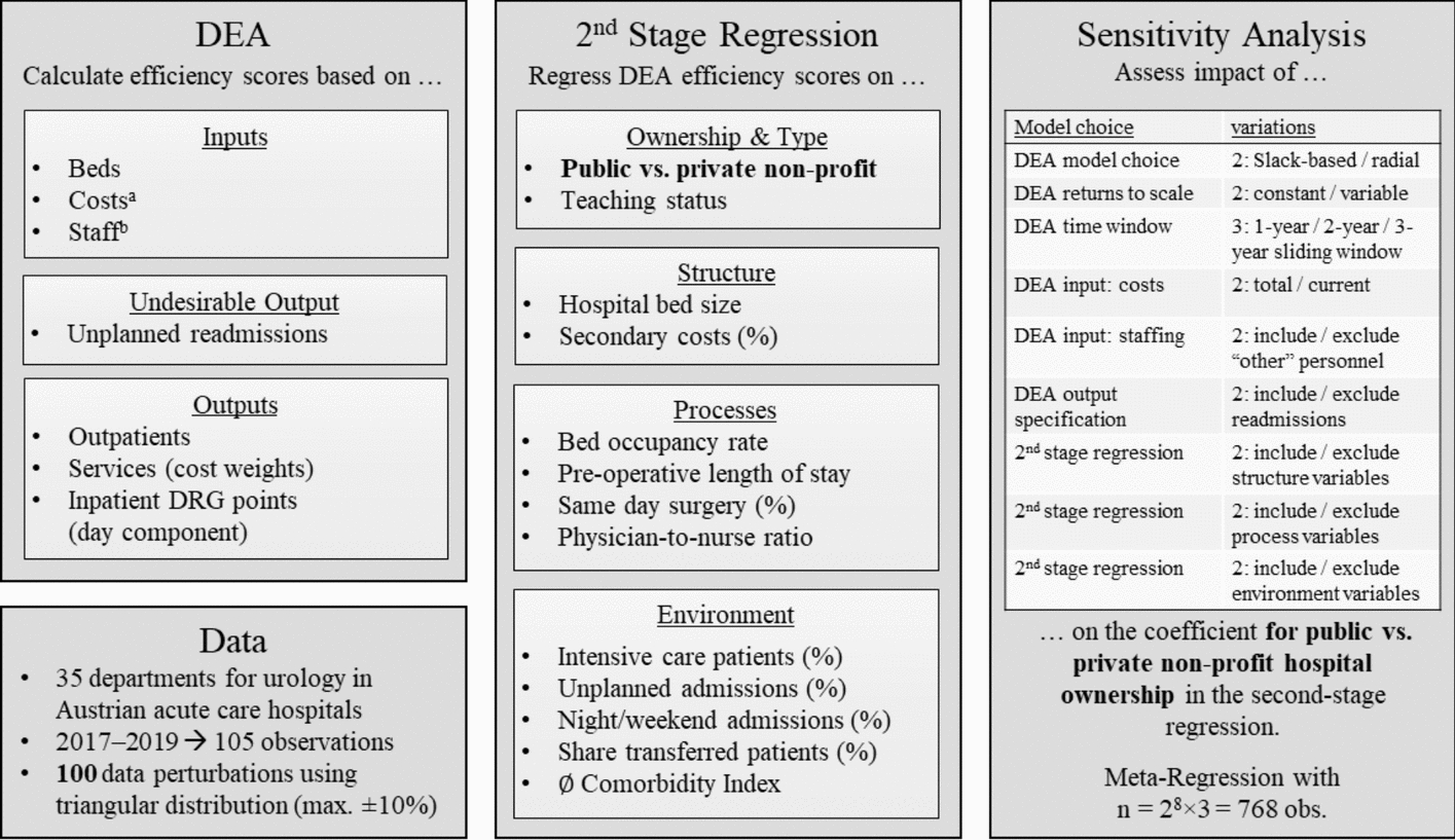
Annex1.1 Measuring inputs and outputs of departments for urology

In the Austrian LKF system, DRG points are defined for the full inpatient episode. The challenge therefore is to isolate the output of specific departments.

1.1.1 Function codes

Function codes can be used to identify specific wards in the LKF dataset and the hospital accounting dataset. The function code has eight digits. The first digit identifies the type of cost-centre, and distinguishes between main, ancillary, and auxiliary cost centres. The second digit identifies, for main cost centres, the type of services that are provided to patients, i.e., whether it is an inpatient ward, whether diagnoses, therapies, and intensive care are provided. Inpatient wards can be identified by having a second digit of < 7, outpatient wards have ≥ 7. The third and fourth digits identify the speciality of the ward. 34 is the code for urology. Finally, the fifth and sixth digits identify specific subspecialities or functions. For example, 11 denotes general urology, 12 denotes andrology, 14 denotes paediatric urology, 15 identifies the lithotripter cost-centre, 81 identifies intensive care units, and 95 identifies operating rooms. The seventh and eight digits allow distinction between cost-centres with identical figures in the previous six digits.

Therefore, urological inpatient wards of a given hospital have function codes of 1 × 34yyzz, where x is < 7, yy is 11, 12, 14 or 81 and zz is any number. Urological outpatient wards follow the same rule, except that x ≥ 7, and yy cannot be 81. Operating rooms can likewise be identified using the appropriate function codes.

Note however that some operating rooms used by urology patients may be operating rooms shared between two or more specialities. These operating rooms do not have 34 (urology) at digits 3 to 4, but rather 91 (interdisciplinary) or 99 (other) and were excluded for this analysis. Their costs and their outputs were not considered.

1.1.2 Beds

The input variable beds is directly extracted from hospital accounting data, i.e., by summarising the number of existing beds in inpatient cost-centres of the relevant speciality.

1.1.3 Staffing

The number of full-time equivalents of various types of personnel is available in the hospital accounting data. we use full-time equivalents weighted by Austrian average of personnel expenditure by full-time equivalent of a given profession, in order to eliminate wage differences between departments that may arise due to differences in the number of years a person has been employed.

Staffing of the category “other” and “operational staff”, which comprise administrative and non-medical technical staff, were excluded, because many hospitals have separate cost centres for these groups of personnel and do not account for them in the urological cost centres. They are included in a version of the sensitivity analysis (see 9.2.7).

1.1.4 Costs (excl. staffing)

Hospital accounting data includes various cost categories. The variable ‘costs’ is created from the sum of cost categories with certain exceptions:

Personnel costs, because staffing is accounted for differently

Costs for services provided by other cost-centres, because these are not included in the output of the urological department (e.g., shared operating rooms)

Energy costs, because of poor data quality and presumed high variance between hospitals

Imputed costs (these are included in the alternative specification of the cost input in the sensitivity analysis, see 9.2.6)

All costs were deflated to 2017 price basis using CPI.

1.1.5 Outpatients

The number of patients treated in a given cost-centre per year is recorded in the hospital accounting data. Therefore, the number of patients treated in a hospital outpatient ward can be directly extracted from the hospital accounting data.

This data could also be extracted from the LKF dataset, which has data on both outpatients and inpatients. But, for inpatients, it only includes wards (i.e., units with beds). Therefore, if a patient is treated in an outpatient ward and later admitted to the hospital, the information on the visit of the outpatient ward is discarded. In order to accurately reflect the patient load of the outpatient ward, we therefore draw upon the hospital accounting dataset to obtain the number of patients that pass through outpatient wards by summarising the number of inpatients and outpatients in urological outpatient wards.

1.1.6 DRG points, day component

For most inpatient episodes, i.e., excluding rehabilitation or psychiatry, the DRG score consists of day components and service components.

The day component is assumed to cover costs of ongoing care, including medication (except for high-priced drugs). The amount depends on the length of stay, but in order to incentivise shorter stays a non-linear mechanism is in effect. For a reference period that is defined for every DRG node, the day component is fixed. For every day in excess or short of that period, points are added or subtracted (Hagenbichler 2010).

A service component covers costs of specific services typically rendered to patients that fall within the DRG node. The LKF system includes rules that govern the amount of DRG points that are awarded if the service is performed multiple times, or if additional services are performed.

Inpatient episodes with stays in intensive care units are awarded additional points based on the number of days spent in these units.

Since the LKF dataset also contains data about the days spent in various types of wards, the day component can be allocated to the wards a patient passes during an inpatient stay by weighting the day component of the DRG score by the share of days a patient has spent in the relevant ward.

For example, in order to calculate the day component DRG points for a department of urology, I summarise the day component of all patients that have ever passed a urological inpatient ward during their inpatient episode multiplied with the share of days that were spent in a urological ward. If patients spent the whole inpatient episode in a urological ward, that share equals 1.

Since there are no urological intensive care units in Austrian acute care hospitals, information on intensive care during the inpatient stay is limited to the second stage regression.

Likewise, intensive care points can be attributed to wards of a speciality by summarising intensive care points of all patients that have passed a urological intensive care ward, applying weights as share of intensive care days that were spent in urological intensive care units.

1.1.7 Services

The LKF dataset also contains services provided to patients along with the function code of the cost-centre that provided the service, service provision can be attributed to the relevant providers by summarising the services produced by the relevant cost-centre. Services provided by shared operating rooms, or other specialities, have the function code of the relevant cost centre that provides the service. These services are not included as outputs of the urological departments, and costs internally billed for provision of this services are excluded from the cost figure (see above).

1.1.8 Readmissions

Readmissions were calculated using the LKF dataset. It contains a patient identifier that allows tracing patient careers over time. For this analysis, readmissions must adhere to the following criteria.

In order to avoid mixing shares and absolute values in DEA inputs (Kohl et al. 2019), the absolute number of readmissions was included as an undesirable output.

1.2 Mathematical specification of the applied methods1.2.1 Perturbation of data using triangular distribution

To assess the robustness of our efficiency estimates to potential data inaccuracies, we implemented a data perturbation bootstrapping approach following the recommendations of Tone (2013). Instead of resampling observations, this method involves perturbing the values of all input and output variables in the original dataset. For each of the 100 bootstrap iterations, every input (staffing, beds, costs, readmissions) and output (DRG points, services, outpatients) value was multiplied by a random scaling factor drawn from a triangular distribution with a lower limit of 0.90, an upper limit of 1.10, and a mode of 1.00. This scaling effectively introduces random noise of up to ± 10% to the original data, simulating potential measurement errors or data variations.

1.2.2 Sliding time windows

The baseline DEA model employed a 2-year sliding window approach to calculate efficiency scores across the study period (2017, 2018, and 2019). This method involved calculating three distinct sets of efficiency scores:

Set 1 (2017–2018): DEA was performed using data from 2017 and 2018.

Set 2 (2017–2019): DEA was performed using data from 2017, 2018, and 2019.

Set 3 (2018–2019): DEA was performed using data from 2018 and 2019.

The efficiency score for a unit o in year t is thus given by

$$_^=\left\_^ \quad if \,t = 2017\\ _^ \quad if \,t = 2018\\ _^ \quad if \,t = 2019\end\right.$$

where \(_^}_-}_\right)}\) denotes the efficiency score of unit o in year t calculated using the DEA model with data from year y1 to y2.

This 2-year sliding window approach was chosen as a balanced trade-off between maintaining a sufficient number of observations within each DEA run to ensure a robust frontier estimation and accounting for potential shifts in regulatory or operational conditions over the three-year period. Data beyond 2019 were not included in the analysis due to the significant and potentially distorting impact of the COVID-19 pandemic on hospital operations, making comparisons with the pre-pandemic period less meaningful.

To assess the sensitivity of the results to the chosen window length, two alternative specifications were also analysed (see 9.2.7):

3-Year Window: Using only the efficiency scores derived from the full three-year dataset (Set 2) for all years: ρ \(_^=_^\)

1-Year Window: Calculating DEA efficiency scores separately for each year using only the data from that specific year.

This approach is consistent with recommendations in the DEA literature for addressing temporal dynamics in efficiency analysis (Alkhars et al. 2022).

1.2.3 Slack-based measure of (super-)efficiency

The DEA analysis is performed using the slacks-based measure of efficiency, as specified by Tone (2001). It calculates efficiency of unit o, \(_\), by minimizing input slacks as a ratio of total inputs \(\frac_^}_}\) as well as output slacks as a ratio of total outputs \(\frac_^}_}\) for all inputs \(i=1,\dots ,m\) and outputs \(r=1,\dots ,s\).

$$_=\underset^,^}}\frac_^\frac_^}_}}_^\frac_^}_}}$$

Subject to

$$_^__+_^=_,i=1,\dots ,m$$

$$_^__-_^=_,r=1,\dots ,s$$

where \(_\) is the weight of the relevant unit j in forming the efficiency frontier, and \(_^__\) is the relevant point of the efficiency frontier for input i.

The input-oriented efficiency score is given by minimizing the input slacks only, specifying that the outputs must remain at the same level:

$$_^=\underset^}}\left(1-\frac_^_^\frac_^}_}\right)$$

Subject to

$$_^__+_^=_,i=1,\dots ,m$$

$$_^__\ge _, r=1,\dots ,s$$

This method is implemented in the function `model_sbmeff` in the R-package deaR (Coll-Serrano et al. 2023).

For efficient units, we use the slacks-based measure of super-efficiency, as proposed by (Tone 2002). It is calculated by eliminating the unit under investigation from the reference set. The objective function minimizes superslacks as share of inputs \(\frac_^}_}\) and outputs \(\frac_^}_}\), respectively.

$$_=\underset^,^}}\frac_^\frac_^}_}}_^\frac_^}_}}$$

Subject to

$$_^__-_^\le _,i=1,\dots ,m$$

$$_^__+_^\ge _,r=1,\dots ,s$$

That is, super-slacks are defined as an input quantity that could be added, or an output quantity that could be removed, under the condition that the unit under investigation o reaches at least the same output and requires up to the quantity of inputs as the reference set, given by \(_^__\) and \(_^__\), respectively.

In the input-oriented version, the objective function operates on input superslacks only and can be expressed as:

$$_^=\underset^}}\left(1+\frac_^\frac_^}_}\right)$$

This method is implemented in the function `model_sbmsupereff` in the R-package deaR (Coll-Serrano et al. 2023).

Note that the additive super-efficiency measure described by Du et al. (2010), which in general minimizes

$$}\frac\left(_^\frac_^}_}+_^\frac_^}_}\right)$$

transforms to a mathematically equivalent minimisation problem under the condition \(_^=0\) (i.e., input-orientation).

1.2.4 Radial measure of (super-)efficenicy

In order to test the sensitivity of results, we switch the efficiency model to the radial (super-)efficiency measure proposed by Andersen and Petersen (1993), who proposed to analyse the efficiency of units that lie on the efficiency frontier radial efficiency models by excluding the unit under investigation from the reference set.

The input-oriented efficiency score is thus calculated by solving the following optimisation problem

Subject to

$$_^__\le\uptheta _,i=1,\dots ,m$$

$$_^__\ge _,r=1,\dots ,s$$

$$_\ge 0,j=1,\dots ,o-1,o+1,\dots ,n$$

\(\sum_^_=1\) for variable returns to scale specifications.

It is implemented in the function model_supereff of the R-package deaR (Coll-Serrano et al. 2023).

Note that, because exclusion of the unit under investigation does not change the efficiency frontier for inefficient units, this model also calculates valid efficiency scores for units with efficiency below 1.

1.2.5 Infeasibility of super-efficiency scores

Given that super-efficiency scores are calculated towards a frontier that is constructed from the set of units excluding the unit under investigation, the variable returns to scale assumption in combination with oriented models may result in a situation in which no units remain in the reference set.

The fact that for these outlier units, efficiency scores cannot be calculated is thus no mathematical shortcoming of the method but an inherent property of the concepts of super-efficiency, orientation, and variable returns to scale in DEA.

To avoid bias in the second-stage regression and meta-regression that would arise from the exclusion of units with infeasible efficiency scores, we use multiple imputation with chained equations (van Buuren and Groothuis-Oudshoorn 2011). We impute these scores based on the inputs and outputs of the units, as implemented in the `mice` package in R.

In the meta-regression, additional covariates count the number of public and private units that were imputed due to infeasibility. This aims to capture potential bias resulting from the imputation.

1.2.6 Second stage regression

The second stage regression serves to explain the efficiency scores as obtained by the DEA based on a set of structure, process and environment covariates.

On the left-hand side of the equation are the efficiency scores. For inefficient units, we use the slack-based measure of efficiency, and for efficient units, we use the slack-based measure of super-efficiency (see Slack-based measure of (super-)efficiency). Explanatory variables are listed in Fig. 1, middle panel.

We calculate an OLS regression model, with the basic form:

$$_=_+_yea_+_publi_+_teachin_+_st_+_pro_+_envi_+_$$

where \(_\) is the (super) efficiency score of unit u, \(_\) is the intercept, \(_\) is a vector of time coefficients, \(_\) is the coefficient that measures the ceteri paribus efficiency difference between units in private non-profit vs. public hospitals, \(_\) is the coefficient that measures the ceteri paribus efficiency difference between units in teaching vs. non-teaching hospitals, \(_\) to \(_\) are vectors of coefficients for structure, process, and environment coefficients respectively, and \(_\) is the idiosyncratic error term.

Models 2 to 4 in Table 3 are versions of this regression, where only one of the groups of structure, process or environment covariates are included in the regression equation. Model 1 only features the intercept and dummy variables for the reference year, public ownership, and teaching status.

We calculate an Ordinary Least Squares (OLS) regression model to estimate the relationship between these covariates and the efficiency scores. Given that the super-efficiency scores used as the dependent variable can exceed 1 and are well above zero, the typical concerns associated with a bounded dependent variable in OLS regression are less pronounced in this analysis. We further address potential heteroskedasticity by calculating heteroskedasticity-robust standard errors (type HC3) using the jtools R package (Long 2024).

The coefficients estimated for the environment covariates, \(_\), in Model 4, Table 3, are used to offset the effects of the external environment in a counterfactual scenario, allowing for a comparison of urology departments under more homogeneous patient structures:

$$_^=_-_\left(envi_-\widehat\right)$$

where \(\widehat\) is the vector of average values of environment covariates.

1.2.7 Sensitivity analysis meta-regression

To assess the sensitivity of the estimated efficiency difference between public and private urology departments to various modelling choices in the DEA and the second-stage regression, a meta-regression analysis was conducted. The dependent variable in this meta-regression was the coefficient for the “public” ownership status dummy variable obtained from each of the \(i = 1, \dots , 768\) individual second-stage OLS regressions that follow various DEA models.

The meta-regression aimed to explain the variation in these “public” coefficients as a function of the specific modeling decisions made in the preceding steps. The general form of the meta-regression model can be expressed as:

$$ \begin \overset$}} _} = \gamma _ + \gamma _ READ_ + \gamma _ DEA_ }} + \gamma _ CONTROLS_ \hfill \\ \quad + \gamma _ \left( \otimes CONTROLS_ } \right) + \gamma _ imputed_} + \gamma _ imputed_} + \in _ \hfill \\ \end $$

where

\(\widehat_}\) is the coefficient of the dummy variable denoting publicly operated hospitals in the second stage regression in the ith second stage regression (see 9.2.6),

\(_\) is the intercept,

\(REA_\) is a dummy variable that equals 1 if unplanned readmissions were included in the DEA specification and 0 otherwise; \(_\) is it’s coefficient

\(DEA\_SPE_\) is a vector of three binary and one ternary variables that describe further specifications of the DEA model, and \(_\) is the relevant vector of coefficients, i.e.

o

Choice of efficiency measure (slack-based vs. radial, see Slack-based measure of (super-)efficiency and Radial measure of (super-)efficenicy)

o

Choice of sliding time window (1 year, 2 years, 3 years) see Sliding time windows

o

Specification of the cost input (see Costs (excl. staffing))

o

Specification of the staffing input (see Staffing)

o

Specification of the returns of scale (see Slack-based measure of (super-)efficiency and Radial measure of (super-)efficenicy)

\(CONTROL_\) is a vector of indicator variables representing the inclusion of different groups of covariates in the second-stage regression (procedure, structure, environment, see Fig. 1). \(_\) is the corresponding vector of coefficients.

\(REA_\otimes CONTROL_\) represents the Kronecker product of \(REA_\) and the \(CONTROL_\) vector, allowing for interaction terms between the unplanned readmissions specification in the DEA and the inclusion of control variable groups in the second stage. \(_\) is the relevant vector of coefficients.

\(impute_\) and \(impute_\) are variables that describe how many public and private units had their super-efficiency score imputed because it was infeasible (see 9.2.5).

\(_\) is the error term for the ith observation, i.e., the ith second stage regression.

The meta-regression was estimated using a fixed-effects model in the metafor R package (Viechtbauer 2010) to assess the overall impact of these methodological choices on the estimated public–private efficiency differential. In the meta-regression, the accompanying variance of \(\widehat_}\), \(_\) was specified as the square robust estimates of standard errors (see 9.2.6). Regressions with more precise estimates (i.e., smaller standard errors and thus smaller variances) are given greater weight in the meta-regression analysis. This ensures that the overall findings of the meta-regression are more influenced by the more reliable individual regression results. The meta-regression was estimated using a fixed-effects model to assess the overall impact of these methodological choices on the estimated public–private efficiency differential, assuming a common underlying true effect.