Appendix A Background on CausalityA.1 Representing Cause-Effect Relationships with Graphs

A graph \(\mathcal = (\textbf, \textbf)\) is a pair of two sets, a set nodes \(\textbf\) and a set of edges \(\textbf \subseteq \textbf \times \textbf\). Two nodes X and Y are adjacent if an edge connects them. Edges can be directed, \(X \rightarrow Y\), or undirected, \(X-Y\). A directed graph is a graph in which every edge is directed. If \(X\rightarrow Y\) then X is a parent of Y and Y is a child of X. A sequence of nodes \(X_1,... , X_k\) form a path if \(X_i\) and \(X_\) are adjacent for every \(i \in [1, k)\). A path is directed if \(X_i \rightarrow X_\) for at least one i [46]. X is an ancestor of Y, and Y is a descendant of X, if there exists a directed path from X to Y. We use An(X) to indicate X’s ancestors, and De(X) to indicate X’s descendants. A cycle is a directed path where \(X_1 = X_k\). A graph is acyclic when there are no cycles. A DAG is a directed and acyclic graph.

Definition 1

(Causal graph) A causal graph (CG) [5] is a DAG \(\mathcal =(\textbf, \textbf)\) where each node \(X_i \in \textbf\) represents a random variable. It is determined by a function \(f_i\) and a set of exogenous variables \(\textbf_X\) so that:

$$\begin X_i := f_i(Pa(X_i), \textbf_X) \end$$

(A1)

with \(Pa(X_i)\) being the parents of \(X_i\).

The exogenous variables indicate the conditions of the world outside the system and are influenced by external factors. Typically, these variables represent the individuals involved in the phenomenon, belonging to the population under study [5]. Hereafter, we refer to the parents \(Pa(X_i)\), including the variables \(\textbf_X\).

A causal graph describes how a system under study works: for each edge \(X \rightarrow Y\), the node X is the cause of Y and Y the effect of X [60]. Observational data are collected without intervening on causal mechanisms [60]. The causal networks framework [5, 59] allows us to relate a causal graph to the data distribution.

Definition 2

(Causal network) A causal network (CN) is a tuple \((\mathcal , P)\) where \(\mathcal =(\textbf, \textbf)\) is a causal graph and P is a joint probability distribution over \(\textbf\) that factorizes into local distributions accordingly to \(\mathcal \):

$$\begin P(\textbf) = \prod _} P(X_i|Pa(X_i)) \end$$

(A2)

The condition in Eq. A2 makes the CN a Bayesian network, where edges also have a causal interpretation [46, 62]. Hence, CNs provide a causal and a probabilistic explanation of the system’s behavior.

Definition 3

(d-separation) Given a DAG \(\mathcal =(\textbf, \textbf)\), a path \(\pi\) between two nodes X and Y is d-separated [61] by a set \(\textbf\subseteq \textbf\setminus \\) if:

\(\pi\) contains a chain of nodes \(X_ \rightarrow X_i \rightarrow X_\) or a fork \(X_ \leftarrow X_i \rightarrow X_\) such that \(X_i \in \textbf\), or

\(\pi\) contains a collider \(X_ \rightarrow X_i \leftarrow X_\) such that \(X_i \notin \textbf\), and no descendant of \(X_i\) are in \(\textbf\).

Two disjoint sets of nodes \(\textbf\) and \(\textbf\) are d-separated by \(\textbf\subseteq \textbf \setminus \, \textbf\}\) if all pairs \((X, Y) \in \textbf \times \textbf\) are d-separated by \(\textbf\). In that case, we write \(\textbf \perp \!\!\! \perp _} \textbf \mid \textbf\).

We denote by \(\textbf \perp \!\!\! \perp _\textbf \mid \textbf\) the conditional independence between the sets of random variables \(\textbf\) and \(\textbf\) given the set \(\textbf\), i.e., whenever \(P(\textbf \mid \textbf, \textbf) = P(\textbf \mid \textbf)\). The condition in Eq. A2 is equivalent to the following Markov property [46, 48]:

$$\begin \textbf \perp \!\!\! \perp _} \textbf \mid \textbf ~\Rightarrow ~ \textbf \perp \!\!\! \perp _\textbf \mid \textbf \end$$

(A3)

The Markov property allows us to read conditional independencies from the graph. However, many DAGs can encode the same set of d-separations. The DAGs that entail the same independencies of a given CG \(\mathcal \) belong to the same Markov equivalence class (MEC) of \(\mathcal \), denoted by \([\mathcal ]\) [62]. A MEC can be uniquely represented by a completed partially DAG (CPDAG), namely an acyclic graph containing directed and undirected edges, in which an edge is directed iff it is directed in all DAGs belonging to the MEC.

A.2 The Problem of Causal Discovery Definition 4

(Causal discovery problem) Let \(\mathcal \) be a dataset over variables \(\textbf\), and \((\mathcal , P)\) the CN that generated \(\mathcal \). The causal discovery problem consists of recovering the CG \(\mathcal \) from data \(\mathcal \) and prior knowledge [31, 77, 93].

Given the true CG \(\mathcal =(\textbf, \textbf)\), a common assumption is that of causal sufficiency, although implausible in many scenarios [45]. Causal sufficiency holds when each variable that causes at least two other variables is observed. When this is not the case, we say there exists at least one unmeasured confounder which is the parent of at least two other observed variables.

There are two main categories of causal discovery algorithms, namely score-based and constraint-based [31, 87, 93]. Score-based algorithms aim to find a DAG \(\mathcal ^*\) that maximizes a goodness-of-fit function, called the score-function. Constraint-based algorithms exploit conditional independence tests to learn the graph’s adjacencies and to orient as many as possible. There is no agreement on which of the two categories is the best in the scientific literature. However, Scutari et al. [73] show that constraint-based approaches perform better in small sample size settings. Another important aspect is that causal discovery algorithms typically do not recover a unique CG, but an MEC, when only observational data are available. Experimental data usually give additional information, allowing us to identify a unique CG [11, 41], but their collection is not always feasible. In this work, we focus on the setting where only observational data are available and resort to expert knowledge for obtaining a unique CG [24].

A.3 Formalizing Expert Knowledge

Expert knowledge, or prior knowledge, is any information that constraints or guides the causal discovery algorithm, typically obtainable from domain experts. There are several approaches to formalize expert knowledge (Section “Related Work”); in this paper, we focus on hard constraints [18], namely, rules on the presence/absence of specific edges in the CG. We denote prior knowledge in this form as \(\mathcal \) [54]. Some constraints are reported in Table 3; it is straightforward to include each rule in constraint-based CD methods [54]. Note that rules 4-8 can be transformed into rule 3. When the number of nodes increases, the edges grow exponentially, making edge-by-edge elicitation unfeasible. On the contrary, partial orders such as rules 5 and 6 are easier to elicit because they describe partial temporal orderings.

Table 3 Examples of prior knowledge constraintsA.4 Estimating Uncertainty in Causal Discovery

Once the causal discovery problem has been solved, the quality of the recovered CG must be assessed. This task may be accomplished by bagging [27], which essentially aggregates a set of CGs learned from sampled subsets of the original dataset. Specifically, let \(\mathcal \) be the true CG and \(\mathcal \) the one learned from data \(\mathcal \). Bootstrap aggregation, abbreviated in bagging, produces many samples \(\_1,..., \mathcal _k\}\) from \(\mathcal \), with or without repetition of data items. In this way, it simulates datasets with a slightly different joint distribution of variables. The sampling technique can also be conditioned on some variables’ values whenever their prevalence is low in \(\mathcal \). Then, a CG is learned from each sample, resulting in a set of graphs \(\_1,..., \mathcal _k\}\). The probability that X and Y are adjacent in \(\mathcal \) is estimated as their adjacency frequency in \(\_1,..., \mathcal _k\}\). A threshold t can be chosen so that edges in \(\mathcal \) are kept only if their probability is higher than t. The value of t may be estimated from data, and a common choice is based on the cumulative distribution function of the empirical probabilities [72]. The probability of edge directions is estimated similarly and selected whenever above 0.5. The empirical probabilities behave as a posterior distribution of \(\mathcal \) given \(\mathcal \). We can then evaluate the robustness of \(\mathcal \) and its generalizability to new data.

Appendix B Longitudinal DataB.1 Notation

Longitudinal data consist of repeated observations of a cohort of individuals over time, hence are characterized by a set of events \(\mathcal \) [55]. An event \(E \in \mathcal \) is any fact that may happen during the patient’s observation period. For instance, it can be the onset of the disease, its progression, or its prognosis. Let \(t=0\) be the initial time point of any observation period [80]. The time at which an event E occurs is said to be its time-to-event \(T^E\). Longitudinal studies aim to model the event-related risk and the cumulative probability distribution of \(T^E\). A subject i is observed up to time \(T_i\), throughout a set of follow-up (FUP) visits which may record event occurrences [78]. The step function \(E_i(t)=\mathbb (T^E_i\le t)\) describes whether E occurred before time t for the i-th subject, with \(0\le t \le T_i\) and \(\mathbb \) the indicator function, which is 1 if the argument is true and 0 otherwise. Note that the \(T_i\)’s are commonly heterogeneous across patients; even if an event has not occurred within the last recorded FUP, we cannot conclude that it will not happen afterwards. This is particularly true in the case of competitive events. For instance, the death event S is competitive when it prevents the observation of subsequent events unless it is the primary focus of the study. The meaning of \(T^S_i\) and \(S_i(t)\) follow from \(T^E_i\) and \(E_i(t)\). A time-to-event \(T^E_i\) is said to be right-censored if \(T^E_i> T_i\). We say the i-th patient is right-censored when \(T^S_i\) is right-censored; this may happen when the subject leaves the study. Classical analysis for these data involves, for instance, the Kaplan-Meier estimate [66] or the Cox Proportional Hazard model [26] in case patients’ covariates and multiple events are considered.

B.2 DataWindowing: A Practical Approach to Time-Varying Mechanisms

We present the DataWindowing algorithm, a preprocessing step to causal discovery tailored for observational longitudinal data.

Let \(\mathcal \) be a dataset in which each row is associated with a subject \(i\in \\) and each column is associated with the observations of either a non-event variable, i.e., determined at \(t=0\) for any i, or an event variable. An event variable related to \(E\in \mathcal \) is the stochastic process E(t) expressing the probability that \(T_E<t\), with \(t>0\). The related column in \(\mathcal \) is:

$$\begin E(T_i)=\left\\right\} \end$$

(B4)

Analogous definitions follow for the stochastic process S(t) and the column \(S(T_i)\), related to the death event S. Notice that E(t) depends on t, hence, E(t) is well-defined for the i-th subject only over \(t\le T_i\). Consequently, there may not exist a unique time \(\tau\) for which \(E(\tau )\) is well-defined for any subject. However, there are no multiple versions of the same node in a CG. Our proposal tackles the issue by removing the dependency of E(t) and S(t) on t.

Let \(\tau> 0\) be a fixed time-point. Algorithm 1 builds a dataset \(\mathcal ^\) from \(\mathcal \), recording whether the events occurred within the time window \([0,\tau ]\). Alive subjects observed less than \(\tau\) are removed from \(\mathcal \) in Lines 5-6. The right-censoring justifies this; we cannot know whether they died within \((T_i,\tau ]\). On the contrary, all those who died before \(\tau\) are kept to avoid selection biases [38]. Here, \(T_i = T_i^S\), so all the event occurrences are recorded at \(T_i\). Each column \(E(T_i)\) is substituted with the realisations of the new variable \(E(\tau )\) in Line 9. If the i-th patient died within \([0,\tau ]\) then \(E_i(\tau )\) is set as \(E_i(T^S)\); otherwise, \(E_i(\tau )\) is set to zero. This way, event variables are given a shared temporal semantics: while E(t) depended on t, now \(E(\tau )\) does not. The same argument holds for the death event S and the column \(S(T_i)\). We do not distinguish between disease-related death and death from other causes.

Follow-ups may be several months apart. If the last FUP is near the selected \(\tau\) for subject i-th, namely \(\tau - \varepsilon \le T_i \le \tau\) with \(\varepsilon\) relatively small, then the next FUP will probably be after \(\tau\). Hence, including i in \(\mathcal ^\) is sensible and increases the sample size. Experts may provide a value for \(\varepsilon\) in Line 4, which depends on (i) \(\tau\) because FUP frequency usually drops over time, and on (ii) i because high-risk subjects are checked more often than low-risk ones.

The choice of \(\tau\) requires a trade-off and relies on experts. The smaller the time window is, the higher the related sample size. On the other hand, time is needed for the events to develop: a small \(\tau\) could hide some cause-effect relationships, because event variables may influence each other from before to after \(\tau\).

Multiple values \(\tau _1<...< \tau _k\) result in different datasets \(\mathcal ^,..., \mathcal ^\) representing the system over overlapping time windows \([0, \tau _1],..., [0, \tau _k]\). Then, the CGs \(\mathcal ^,..., \mathcal ^\) can be learned from them through shared or non-shared prior knowledge. When compared, the CG structures may allow experts to deduce whether, and how, causal mechanisms change over time. Edge removals, additions, and reversals hint that the data-generating process develops over time.

Appendix C Case StudyC.1 Sensitivity Analysis

We perform sensitivity analysis [95] to validate the robustness of the causal sufficiency assumption, specifically regarding the edge from Metastasis to Recurrence.

In epidemiology, sensitivity analyses typically consider the risk ratio (RR) as the causal effect of a treatment on an outcome, then compute indicators of how such an effect is sensitive to the presence of unobserved confounders. One of the most used indicators is the e-value, which assesses the robustness of the effect due to possible unmeasured confounders. According to VanderWeele and Ding [84], the e-value is “the minimum strength of association, on the risk ratio scale, that an unmeasured confounder (Appendix A) would need to have with both the treatment and outcome, conditional on the measured covariates, to fully explain away a specific treatment–outcome association”. Therefore, the higher the E-value, the stronger the confounder associations must be. Additionally, the e-value requires minimal assumptions, e.g., it is independent of the nature of the unobserved confounders [95].

Therein, we consider Metastasis as the treatment and Recurrence as the outcome variables. Hence, the RR compares the risk of occurrence of local recurrence between two groups: those affected by a metastasis and those not affected by it. To estimate such an effect, we rely on the backdoor criterion [62] for each CG. Then, the respective e-values are computed.

Table 4 presents the results.

Table 4 Relative risks and related e-values for each time window

RR lower refers to the lower bound of the 95% confidence interval estimated for the RR, whereas E-value lower if the e-value related to RR lower.

The e-value related to the 0-2 years time window is 8.21, meaning that, given the existence of a biological factor as an unobserved confounder, it must increase both the risk of metastasis and local recurrence by about 8 times, independently of the other covariates, to explain the RR between metastasis and recurrence. Even considering RR lower, the e-value remains quite large. Notice that such a biological factor should be independent of all other covariates, while clinical experts support Grade and Histotype as the two major indicators of tumor aggressiveness. We thus conclude that it is implausible that an unmeasured confounder could explain away the causal effect, thus supporting the validity of the causal sufficiency assumption. Given the large e-values obtained, and supported by the literature [95], we did not conduct any further sensitivity analyses.

C.2 Causal Discovery without DataWindowing

Figure 5 reports the CG obtained by applying a CD algorithm, namely, PC-Stable [17], to the full data set as resulting from step 7, disregarding any time-related information. Doing so, the model loses the ability to describe the disease evolution, thus diminishing its interpretability and utility in practice. Notice that the prior knowledge introduced is the same as the one adopted in the final models, shown in Table 2.

Fig. 5

The CG obtained from the full STS data set, without applying the DataWindowing approach

C.3 Causal Discovery Benchmarking

For benchmarking against the employed PC-Stable algorithm, we consider the score-based TABU [68] and the constraint-based FCI [77] algorithms. Figure 6 outlines the structural differences with what was obtained from PC-Stable. The PC-Stable graphs are taken as ground-truth: red edges are added by either TABU or FCI, whereas dashed blue edges are removed. As the FCI output is an ancestral graph [77], only the presence/absence of edges is directly comparable with other graphs. As for quantitative evaluation and direct comparison, we also report the following structural metrics for the edges: number of true positives (TP), number of false positives (FP), number of false negatives (FN), and the structural Hamming distance (SHD) between graphs [93].

TABU achieves comparable results to those obtained by PC-Stable, however, as noted, such score-based methods hinder a transparent interpretation of the edges in terms of (in)dependences among variables. Thus, it becomes harder to communicate with clinical experts and extract meaningful and sound prior knowledge. Moreover, some relevant edges are missing, such as Margins \(\rightarrow\) LR in \(\mathcal ^2\), which hinders the role of margins, or Histology \(\rightarrow\) DM in \(\mathcal ^2\). However, some added edges may hold an are worth conducting a future analysis, such as Compartment \(\rightarrow\) Margins, holding in every TABU CG. Due to data scarcity, FCI attains only a few edges with plenty of disconnected variables. However, these edges are true positives, namely, a subset of PC-Stable edges. Only in \(\mathcal ^7\) we observe an additional, false positive, edge. Interestingly, LR and DM are always disconnected, perhaps due to the scarcity of those events and their joint observation.

Regarding runtime computation, TABU is the fastest among the others. This is likely due to the conditional independence tests typical of the constraint-based algorithms. However, any algorithm runs in a reasonable time, though constraint-based approaches might not be well scalable on large networks.

Fig. 6

Benchmarking results against PC-Stable

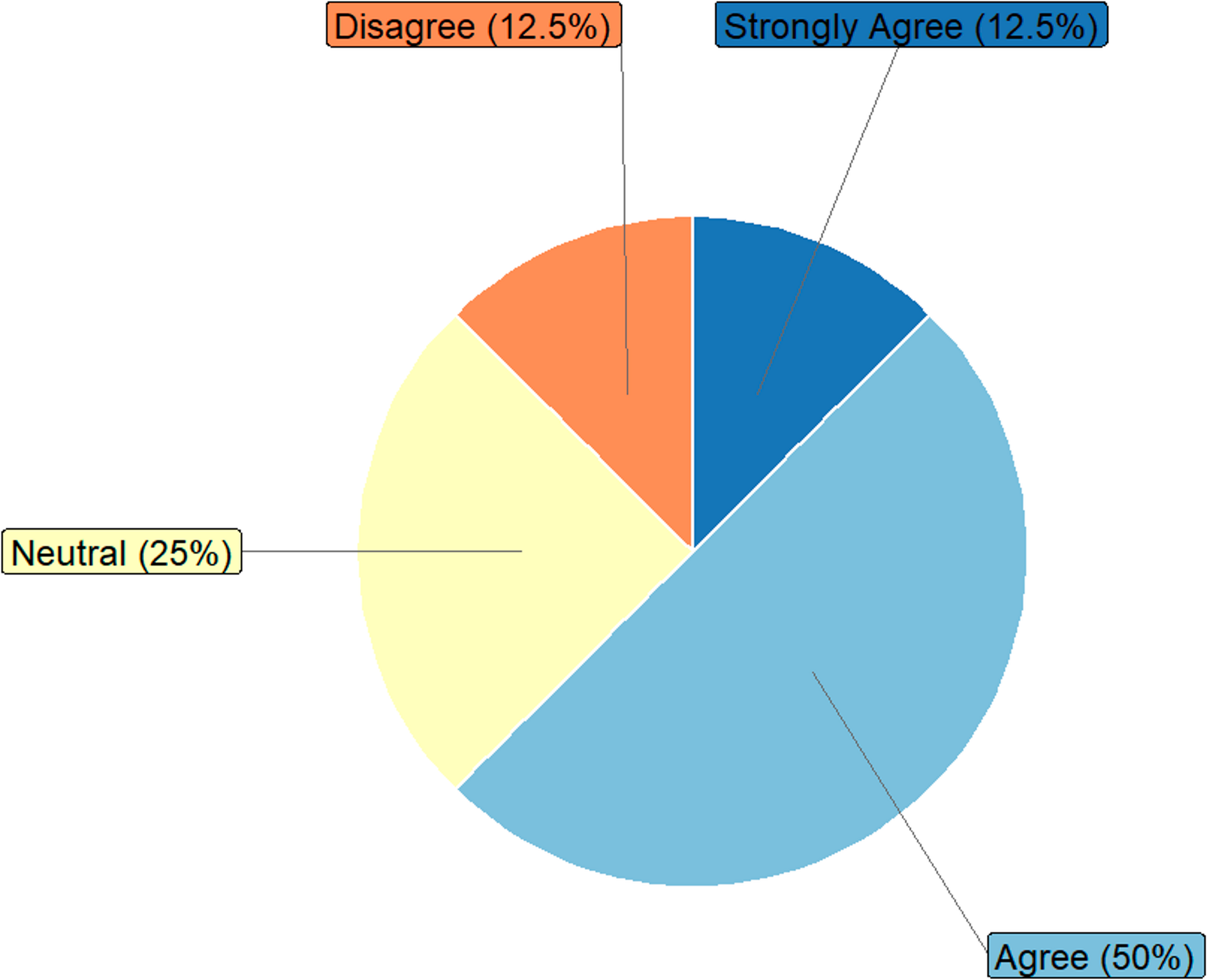
C.4 Questionnaire

For reproducibility purposes, we report the questions in the STS questionnaire. The types and fields of answers are reported for each question. Figures 7, 8, and 9 depict the obtained results.

1.

“Email (optional)”. Free-text input.

2.

“Workplace”. Multiple choice (Oncology/Surgery/Pathological Anatomy/Radiotherapy/Radiology/Other:\(\underline}\)).

3.

“Specialization”. Free-text input (e.g., “Oncologist”, “Surgeon”, etc.).

4.

“Years of experience on soft tissue sarcoma”. Numerical input.

5.

“I took part in this project”. Multiple choice (Yes/No/Other: \(\underline}\)).

6.

“Positive margins (R1 or R2) can cause local recurrence”. 5-point Likert scale + optional comment.

7.

“Positive margins (R1 or R2) can cause distant metastasis”. 5-point Likert scale + optional comment.

8.

“Positive margins (R1 or R2) are also caused by biological variables (e.g., site, histology). If yes, specify which variables”. 5-point Likert scale + optional comment.

9.

“The decision of whether to administer chemotherapy at diagnosis of a STS of a limb or superficial trunk is based on the observation of”. Multiple choice (Never/Rarely/Sometimes/Often/Always) for the following factors + optional comment.

10.

“The decision of whether to administer radiotherapy at diagnosis of a STS of a limb or superficial trunk is based on the observation of”. Multiple choice (Never/Rarely/Sometimes/Often/Always) for the following factors + optional comment.

11.

“Chemotherapy prevents local recurrence”. 5-point Likert scale + optional comment.

12.

“Chemotherapy prevents distant metastasis”. 5-point Likert scale + optional comment.

13.

“Radiotherapy prevents local recurrence”. 5-point Likert scale + optional comment.

14.

“Radiotherapy prevents distant metastasis”. 5-point Likert scale + optional comment.

15.

“Chemotherapy improves patient prognosis in terms of survival”. 5-point Likert scale + optional comment.

16.

“Radiotherapy improves patient prognosis in terms of survival”. 5-point Likert scale + optional comment.

17.

“In the short term (i.e., first 2 years), distant metastasis can cause local recurrence”. 5-point Likert scale + optional comment.

18.

“In the long term (i.e., beyond 5 years), distant metastasis can cause local recurrence”. 5-point Likert scale + optional comment.

19.

“A local recurrence can cause distant metastasis”. 5-point Likert scale + optional comment.

20.

“In the short term, local recurrence can cause patient death”. 5-point Likert scale + optional comment.

21.

“In the long term, local recurrence can cause patient death”. 5-point Likert scale + optional comment.

22.

“In the short term, certain histologies and grading cause distant metastasis”. 5-point Likert scale + optional comment.

23.

“In the short term, certain histologies and grading cause local recurrence”. 5-point Likert scale + optional comment.

24.

“In the long term, histology and grading do not cause local recurrence”. 5-point Likert scale + optional comment.

Fig. 7

Results of the STS questionnaire (first part)

Fig. 8