Design and working principle of the experimental ultrasound setup

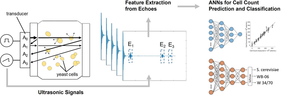
The experimental ultrasound setup consisted of the electronic components used for both ultrasonic signal excitation and acquisition, as well as the sample vessel (see Fig. 1). A Varivent® process connector was used as the sample vessel, suitable for hygienic applications and allowing integration of measurement and control instruments. The stainless-steel sample vessel included two Plexiglas® plates that enclosed the buffer rod (i.e., medium 1) and the parallel reflector (i.e., medium 3); see Fig. 1a. The buffer rod had a diameter, db, of 17 mm, and the sample vessel had a diameter, d, of 37.5 mm. To ensure a leak-tight closure, the bottom of the Varivent® process connection was secured with a blind nut. The waveform generator (Agilent 35522 A, Keysight Technologies, Santa Rosa, CA, USA) produced a 10 Vpp pulse with a four-cycle square wave excitation. This electrical pulse was directly applied to a 2 MHz piezoelectric ultrasonic transducer (MB 2 SE, GE, Boston, MA, USA), which was mechanically coupled to the buffer rod (see Fig. 1b). The transducer functioned as both transmitter and receiver of ultrasonic signals, generating and detecting ultrasonic waves within the experimental setup. The buffer rod served as an acoustic delay line, which enabled transmitting the produced ultrasonic wave into the sample medium (i.e., medium 2) and temporal separation of the echoes. For effective ultrasound transmission into the sample, coupling gel (Aquasonic® 100, Parker Laboratories Inc., Fairfield, NJ, USA) was used. The reflected echoes were captured with the same transducer and recorded directly by an oscilloscope (PicoScope 5204, Pico Technology, Cambridgeshire, UK) without any additional analog amplification or filtering. Data acquisition was performed using PicoScope 6 software (Pico Technology, Cambridgeshire, UK) at a sampling rate of 1 GHz. The schematic configuration and signal path of the experimental ultrasound setup are summarized in Fig. 1c.

Fig. 1

Schematic illustration of ultrasonic wave propagation in the experimental ultrasound setup (a), technical drawing of the sample vessel (b), and flowchart illustrating the ultrasound signal path from excitation to recording of the raw ultrasound data, \(_(t)\) (c). In a, arrows indicate the path of the ultrasonic wave propagation and its interactions with different media. The waveform generator excites the transducer, thereby generating the initial ultrasonic wave with amplitude A0. This wave propagates through the buffer rod into the sample, where multiple reflections and interactions occur. The first echo, E1, arises at the buffer rod–sample interface; the second echo, E2, is generated at the sample–reflector interface; and a third echo, E3, results from the wave traversing the sample a second time. All echoes are captured by the transducer and recorded using an oscilloscope, yielding amplitudes A1, A2, and A3

The cross-sectional schematic of the sample vessel in Fig. 1a illustrates the propagation of the ultrasonic wave through the three sequentially layered media: the buffer rod (medium 1), the yeast suspension sample (medium 2), and the reflector (medium 3). The ultrasonic signal is generated by a 2 MHz transducer, which is excited by the waveform generator. The initial ultrasonic wave, with amplitude A0, propagates through the buffer rod and reaches the buffer rod–sample interface. At this interface, a portion of the wave is reflected, forming the first echo, E1, with amplitude A1, which is received by the transducer without entering the yeast suspension (i.e., sample). The transmitted portion of A0 propagates through the yeast suspension and is reflected at the sample–reflector interface, generating the second echo, E2, with amplitude A2. This echo traversed the sample twice (i.e., a propagation path within the sample of 2d) and carries information about the acoustic attenuation and transmission characteristics of the yeast suspension. A third echo, E3, with amplitude A3 results from an additional reflection cycle within the sample. Due to the extended propagation path within the sample of 4d, A3 experiences greater attenuation and may provide information about multiple scattering effects in the sample medium.

Sample preparation

Wort solutions were prepared with extract concentrations of 10, 12, and 14 wt%. To do this, a commercially available malt extract (Bavarian pilsner, Weyermann® GmbH, Bamberg, Germany) was diluted with demineralized water to the target wort concentrations. The required amount of malt extract was calculated based on the analytically determined concentration of the Bavarian pilsner malt extract.

Three commercially available dry yeast strains, with unique physiological properties and commonly used in the food and beverage industry, were selected for this study. Top-fermenting Saccharomyces cerevisiae (code: S. cerevisiae; FERMIPAN® RED, Casteggio Lieviti srl, Casteggio, Italy) and Saccharomyces cerevisiae var. diastaticus (code: WB-06; SafAle™ WB-06, Fermentis, Division of S.I. Lesaffre, Marcq-en-Baroeul, France) were examined. A bottom-fermenting yeast, Saccharomyces pastorianus (code: W 34/70; SafLager™ W 34/70, Fermentis, Division of S.I. Lesaffre, Marcq-en-Baroeul, France) was also investigated. WB-06 is commonly used for wheat beer fermentation (e.g., hefeweizen or Belgian witbier). In contrast, W 34/70, a natural hybrid of S. cerevisiae and S. eubayanus, is the most widely used lager yeast in the brewing industry. All sealed dry yeast samples were stored at 4 °C until use.

To maintain the original physiological state and morphology of the yeast, and to prevent yeast proliferation and CO2 production during rehydration, dry yeast was first suspended in sterile 25% Ringer solution (i.e., electrolyte solution) for 30 min at 20 °C. Following rehydration, the suspension was centrifuged at 3000 rpm for 10 min at 20 °C. The supernatant was discarded, and the yeast was washed with the corresponding wort and centrifuged again. After washing, concentration gradients were prepared for each yeast by suspending the washed yeast in wort. A concentration gradient from 0.0 wt% to 1.0 wt% was prepared with 0.2 wt% increments, resulting in six concentration levels per strain. These gradients were prepared for each wort concentration (10, 12, and 14 wt% extract); each yeast suspension in the gradient was 250 mL in volume. For all sample increments, yeast cell count was determined using a hemocytometer with a chamber depth of 0.1 mm (Blaubrand, Sigma-Aldrich, St. Louis, MO, USA), following the procedures outlined in MEBAK sections 10.4.3.1 and 10.11.4.4 [38]. All yeast suspensions used in this study were produced in three biological replicates.

Ultrasonic measurements

All samples across the concentration gradient (0.0–1.0 wt%), for each yeast strain at each wort concentration (10, 12, and 14 wt% extract), were measured in the experimental ultrasound setup at 20 °C. At each yeast concentration increment, 50 ultrasound signals were recorded in 0.5 s intervals, resulting in a total acquisition time of 25.0 s. Processing and feature extraction of the recorded raw ultrasound data, \(_(t)\), were carried out as described below.

Ultrasound data processing

Ultrasound data processing was performed using MATLAB R2023a (MathWorks, Natick, MA, USA).

Preprocessing of ultrasound signals

The recorded raw data, \(_(t)\), from the ultrasonic measurements were one-dimensional time series sampled at 1 GHz. To isolate the frequency range most responsive to the transducer, the signals were filtered using an eighth-order bandpass filter centered around 2 MHz (i.e., 1.5–2.5 MHz). Filtering was performed in a zero-phase manner to preserve the temporal structure of the signals and ensure sufficient attenuation of frequency components outside the passband [39]. The resulting filtered time domain signal retained the original echo structure. To enhance the signal-to-noise ratio, every five consecutive signals were averaged. This procedure improved signal consistency and suppressed random fluctuations, resulting in the ultrasound signal, \(x\left(t\right)\); see Fig. 2.

Fig. 2

Representative ultrasound signal, \(x\left(\text\right)\), showing three detected echoes (E1, E2, and E3). The complete signal is shown in a, with the echo locations indicated by boxes. Enlarged views of each echo are included in b. The echoes were identified within predefined time intervals

Ultrasound feature extraction

To identify relevant echo characteristics, the envelope, \(e\left(t\right)\), of each ultrasound signal, \(x\left(t\right)\), was calculated. The envelope, \(e\left(t\right)\), approximates the instantaneous amplitude of the signal and allows robust identification of reflected signal structures [40]. It was estimated by detecting the local maxima of the absolute signal within a moving window of 1000 sample points, which corresponds to 1000 ns at a 1-GHz sampling rate. This method effectively extracts the upper contour of the waveform and accentuates energy-rich regions, such as echoes. Three predefined time intervals, corresponding to the expected echo arrivals, were selected based on prior knowledge of the experimental setup geometry and signal propagation times; see Fig. 2b. The predefined time intervals selected for echo signal characterization were as follows:

First echo, E1: [a1, b1] = [10,000, 15,000] ns

Second echo, E2: [a2, b2] = [60,000, 65,000] ns

Third echo, E3: [a3, b3] = [72,000, 77,000] ns

For each echo i ∈ , the following three temporal and amplitude-related ultrasound signal features were extracted:

The maximum amplitude, \(_\), of the envelope, \(e\left(t\right)\), within the time interval [\(_\), \(_\)]:

$$_=\underset_, _\right]}}e\left(t\right).$$

(1)

The time, \(_\), at which \(e\left(t\right)\) reaches its maximum within the same interval:

$$_=\underset_, _\right]}}\,\, e\left(t\right).$$

(2)

The sum, \(_\), of the absolute values of the signal \(x\left(t\right)\) over the interval, which serves as a measure of signal intensity:

$$_=\sum__}^_}\left|x\left(t\right)\right|.$$

(3)

These ultrasound-derived features provide quantitative and qualitative information about the interaction of ultrasonic waves with the sequentially layered media of the experimental setup. The three recorded echoes differ in their propagation paths and physical origins. Therefore, the derived features (\(_\), \(_\), and \(_\)) capture specific acoustic interactions that depend on the media properties and the corresponding propagation path length. The extracted features of the first echo, E1, mainly represent the acoustic impedance contrast at the buffer rod–sample interface. In contrast, E2 and E3 traverse the yeast suspension and therefore carry information related to the attenuation and scattering properties of the suspension. The maximum amplitudes of E2 and E3 (\(_\) and \(_\)) reflect the local peak signal intensities, with higher yeast concentrations causing stronger attenuation and, consequently, lower amplitudes. Accordingly, the temporal positions of the echo maxima (\(_\) and \(_\)) are associated with the effective speed of sound and acoustic path length within the sample. The sums of the absolute values of E2 and E3 (\(_\) and \(_\)) represent the total reflected acoustic energy, thereby integrating the effects of both attenuation and scattering-related signal broadening. Collectively, these features translate the raw ultrasound signals into quantitative descriptors of the examined yeast suspensions. This procedure yielded three features per analyzed echo, resulting in a total of nine ultrasound-derived features that were used as input features for subsequent model training and development.

Artificial neural networks

Five artificial neural network modeling approaches were developed using MATLAB R2023a (MathWorks, Natick, MA, USA), and these are summarized in Tables 1 and 2. All ANN models were trained on a system equipped with an AMD Ryzen 7 5825U processor (2.0 GHz, 8 cores, 16 GB RAM) without GPU acceleration. Approaches 1–4 focused on predicting yeast cell counts using regression models (Fig. 3a), while Approach 5 was developed for the classification of samples by yeast strain (Fig. 3b). The regression models differed in the manner in which nominal categorical (strain identity) and ordinal (wort concentration) information were incorporated as model inputs. Strain identity was excluded entirely in Approaches 1 and 2 but included as an encoded input feature in Approaches 3 and 4. In Approach 5, by contrast, strain identity was used as the prediction target in a multi-class classification model. However, all ANNs shared the same basic network architecture with two hidden layers and used a data split of 80:20 for training and testing. Model performance was assessed using fivefold cross-validation on the training set and subsequently evaluated independently on the test set.

Table 1 Overview of artificial neural network (ANN) hyperparameters and training settingsTable 2 Overview of the artificial neural network (ANN) approaches usedFig. 3

Comparison of the used basic artificial neural network architectures for regression (a) and classification (b). Both models have an input layer with 9–13 neurons, depending on the number of input features used in each approach (neurons partially shown; represented by gray circles), and two fully connected hidden layers with five and three neurons, respectively. The regression ANNs have a single output neuron suitable for predicting yeast cell count. The classification ANN includes three output neurons with a softmax activation function in the output layer, enabling multi-class classification of the yeast strains

Model architecture and data management

Preliminary modeling included systematic testing of different network depths (1–3 hidden layers), numbers of neurons per layer (5–30), and L2 regularization strengths (λ = 0.0–0.1). Increasing model complexity reduced training bias but led to a widening discrepancy between training and test errors, indicating a tendency toward overfitting. Therefore, a compact, fully connected artificial neural network with two hidden layers (five and three neurons) was selected as the basic network architecture to balance model complexity and generalization performance. The rectified linear unit (ReLU) activation function was applied to all hidden layers. In addition, L2 regularization (λ = 0.001) was applied to all models to prevent overfitting by penalizing large network weights. This regularization term helped stabilize training and improve generalization performance. Prior to training, all ultrasound-derived input features were standardized to zero mean and unit variance. The regression models minimized mean squared error (MSE), while the classification model was trained using cross-entropy loss. Model optimization employed the limited-memory Broyden–Fletcher–Goldfarb–Shanno (L-BFGS) algorithm, and network weights were initialized with Glorot uniform initialization [41]. To prevent overtraining, early stopping with a validation patience of six epochs was implemented, halting training when performance no longer improved. The network architecture, hyperparameters, and training settings used are summarized in Table 1.

For each strain, the dataset used for regression model training included the manually determined cell counts and nine ultrasound-derived features from all individual samples in the yeast suspension concentration gradients, with each sample assessed at three different wort concentrations. These three strain-specific datasets (used in Approach 1) were then merged to form the combined dataset (used in Approaches 2–5). Therefore, the combined dataset consisted of three identically structured sets, each corresponding to a different yeast strain. Approaches 1–4 were developed as regression models for yeast cell count prediction, with Approach 1 trained on strain-specific datasets and Approaches 2–4 trained on the combined dataset. While Approach 2 used only ultrasound-derived features as inputs, Approaches 3 and 4 progressively incorporated additional encoded variables, beginning with nominal strain identity and followed by ordinal wort concentration. In contrast, Approach 5 was developed as a classification model to distinguish between yeast strains. An overview of all approaches is provided in Table 2.

Each dataset (strain-specific or combined), with its respective input features and prediction target, was randomly partitioned into 80% for training and 20% for independent testing (see Fig. 4). Within the training set, fivefold cross-validation was applied to evaluate model performance and generalization. Test data were not used during training, thereby ensuring unbiased model performance assessment. The evaluation metrics used are described in the section “Model Evaluation Metrics.”

Fig. 4

Overview of data partitioning and evaluation procedure. The data (100%) were split into a training set (80%) and a test set (20%). The training set was used for model training with fivefold cross-validation to assess model performance. Final model performance was evaluated on the independent test set

Regression models for yeast cell count prediction (Approaches 1–4) Approach 1: Strain-specific regression

An independent model was trained for each yeast strain, resulting in three separate models for yeast cell count prediction. Approach 1 represents a use case where the strain identity (e.g., W 34/70) is known at prediction time. Therefore, each model was trained independently using only the corresponding yeast strain training set (80% of the data), with the nine ultrasound-derived features as input, each corresponding to one neuron in the input layer. Approach 1 handled three smaller datasets and allowed models to specialize in strain-specific patterns for cell count prediction.

Approach 2: General regression model

In Approach 2, the combined dataset, formed by merging three strain-specific yet identically structured datasets, was used to develop a single regression model able to predict yeast cell count for all strains. This ANN used only the nine input features derived from ultrasound echoes, with the manually determined yeast cell counts as the prediction target. This general modeling approach provided an initial assessment of the predictive power of the ultrasound-derived features alone for yeast cell count prediction. Additional input features, such as strain identity and wort concentration, which represent biological differences and process variability, respectively, were not included.

Approach 3: Regression with one-hot encoding of strain identity

Approach 3 expands on Approach 2 by introducing strain identity as a nominal categorical variable via one-hot encoding [42]. Three binary indicators were used to encode the strain identity: S. cerevisiae as [1 0 0], WB-06 as [0 1 0], and W 34/70 as [0 0 1]. These one-hot encoded vectors added three input neurons to the model and were concatenated with the nine original ultrasound-derived features. Therefore, the regression model of Approach 3 used a total of 12 input neurons. One-hot encoding was chosen since the nominal nature of the strain identity indicates that the classes have no inherent order or hierarchy. Therefore, Approach 3 allowed the model to predict yeast cell counts across all strains while accounting for strain-specific differences.

Approach 4: Regression with one-hot encoding of strain identity and ordinal encoding of wort concentrations

This modeling approach for yeast cell count prediction incorporated two additional non-ultrasound input features: strain identity and wort concentration. Strain identity was treated as a nominal categorical variable and encoded using one-hot vectors ([1 0 0], [0 1 0], [0 0 1]), while wort concentrations of 10, 12, and 14 wt% were encoded as an ordinal variable with values of −1, 0, and +1, respectively. Unlike the nominal nature of strain identity, the ordinal encoding of wort concentration reflects an inherent order. This allowed the model to account for both nominal categorical variation (strain identity) and ordered process variability (wort concentration), thereby improving its ability to learn from the underlying relationships in the data. Therefore, a total of 13 input features were used: nine ultrasound-derived features, three binary indicators for strain identity, and one numeric variable for wort concentration. Each input feature corresponded to one neuron in the input layer. Among the regression models, this configuration provided the highest input complexity and specificity and was expected to improve generalization across different strains and wort concentrations.

Yeast strain classification model (Approach 5) Approach 5: Classification of yeast strains

In this approach, a classification model was trained to predict strain identity (i.e., class membership) based solely on the nine ultrasound-derived features. This model shared the same basic network architecture as Approaches 1–4, but differed in the output layer, which employed a softmax function for multi-class classification of yeast strains (see Fig. 3b). This approach served as a verification model, designed to assess whether the ultrasound-derived features align with the expected strain classification.

Model evaluation metrics

Model evaluation metrics were calculated using fivefold cross-validation on the training set and subsequently evaluated on the independent test set. Cross-validation provided a general estimate of model performance, while the test set allowed for independent assessment of generalization to unseen data. For the regression models (i.e., Approaches 1–4), model performance was assessed using the coefficient of determination (R2), root mean square error (RMSE), and mean absolute error (MAE):

$$^=1- \frac^_-}}_\right)}^}^_-} }\right)}^},$$

(4)

$$RMSE=\sqrt \sum_^_-}}_\right)}^},$$

(5)

$$MAE=\frac\sum_^\left|_-}}_\right|,$$

(6)

where \(_\) is the measured (i.e., true) value, \(}}_\) is the predicted value, \(}}\) is the mean of the measured values, and \(n\) is the number of data points.

For the classification approach (i.e., Approach 5), the model performance was assessed using overall accuracy, defined as the percentage of correct predictions. Additionally, model performance metrics for each yeast strain class, including precision, recall, and F1-score, were calculated as follows:

$$\mathitscore} = 2 \cdot \frac \cdot \mathit} + \mathit}$$

(9)

True positives (TP) indicate the number of instances correctly classified as belonging to their actual yeast strain class, and false positives (FP) represent the number of instances incorrectly classified as belonging to a particular strain when these belong to another. False negatives (FN) are instances from a given yeast strain that were misclassified as belonging to a different strain. These metrics evaluate the performance of the classification model in distinguishing between yeast strains.