Feature extraction and Procrustes analysis

Following parameter optimization for the validation dataset I, five feature peak matrices were generated, each representing 53 samples and varying in feature count: MarkerView (1315), XCMS (280), MZmine3 (315), OpenMS (248), and SIRIUS (166). MarkerView extracted the highest number of features, while SIRIUS extracted the fewest. Targeted analysis using SCIEX OS confirmed the consistent detection of the eight spiked compounds across all pool samples. All software tools, except SIRIUS, successfully captured these targets; SIRIUS failed to detect 2-TFMB, fluopyram, and prometryn. Manual review of feature lists revealed that most software detected key isotopes and adducts linked to the main ion ([M+H]+). 37Cl isotopes of atrazine, clothianidin, and epoxyconazole were present in the feature lists of all software with an exception of MZmine3. However, the 37Cl isotope of fluopyram was absent from the OpenMS and XCMS datasets. For all targets, the [M+Na]+ adduct was included in the feature lists of MarkerView resulting from an improper componentization. Additionally, several adducts and in-source fragments were also present in in this feature list, as reported before [23].

Procrustes analysis was then used to evaluate the alignment between a reference data matrix, containing targeted [M+H]+ features from SCIEX OS (dstd), and feature profiles generated by five software tools across 53 pooled samples. As outlined in Fig. 3, the reference matrix was derived from targeted analysis in SCIEX OS, while the corresponding data matrices were constructed by manually extracting the same target compounds from each software’s feature list. Each matrix was individually compared to the reference. MarkerView exhibited the closest alignment (d = 0.0112), followed by OpenMS (0.0165) and MZmine3 (0.0182). XCMS showed greater dissimilarity (d = 0.0383), partly due to misalignments such as propamocarb duplication. SIRIUS demonstrated the highest dissimilarity (d = 0.2809), indicating the weakest concordance.

Fig. 3

Procrustes analysis comparing each software-derived target matrix (MarkerView, MZmine3, OpenMS, SIRIUS, XCMS) to the SCIEX OS reference

Data exploration of validation dataset IPCA

The initial data exploration was conducted using PCA for each feature list. The five scenarios demonstrate each algorithm’s influence on interpretations. The score and loading scatter plots for each software across PCs 1–4 (Figures S3–S6) show that the first two components mainly capture overall data variation, including instrument- or software-related signal fluctuations and potential sensitivity drifts not fully corrected by IS normalization. In practice, the incomplete IS-based correction was deliberately maintained to assess how different software tools respond to residual signal drift. In contrast, the third and fourth components primarily capture residual variation, including fluctuation and spill-like events introduced by the predefined spiking patterns (Figure S5), with interpretations varying depending on the MS software used (see SI-4.2 and Figure S7 for details).

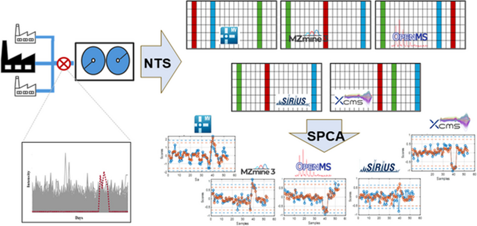
SPCA

Principal components, however, are linear combinations of all variables in the matrix and are therefore difficult to label. In order to enhance the interpretability of scores/loading in a comparative analysis of provided feature lists and overcome limitations of PCA in inferences extracted on high-dimensional data, we suggest implementing sparse factorization methods, such as SPCA. In high-dimensional datasets, SPCA can reduce noise by isolating significant features and suppressing irrelevant ones. In the context of the current time-series LC-HRMS datasets, SPCA enhances component clarity in noisy datasets across various packages and assists in identifying key drivers of various time trends. Weak variable associations and unclear structure in MEDA maps reduce the effectiveness of sparse methods like GPCA or structured SPCA. This contradicts MarkerView, which exhibits clear feature clustering and makes it a suitable candidate for GPCA, as previously reported [23].

Another important superiority of SPCA is the possibility of detecting effective features with different spill structure in one subspace, which is not the case for GPCA, for example. For the current datasets, SPCA is a more suitable alternative as it applies sparsity constraints to select only the most relevant features, leading to a more concise model and improving interpretability without requiring predefined groups. Since the extracted features consist of unique precursors with/without adducts (or fragment), depending on the software, implementation of Elastic Net regularization which incorporates both LASSO (L1) and ridge (L2) penalties allows correlated variables to share influence, often entering the model together. This will allow control of the trade-off between variable selection and multicollinearity. Among SPCA formulations, we adopted the algorithm by Zou [22] and empirically balanced the L1 and L2 penalties for each data matrix to recover targeted features that capture discriminative patterns distinct from the general wastewater profile (see SI-3).

General trend observations

The final results of exploratory analysis of five data matrices using SPCA for first 10 PCs for target detection (true positives) under optimized penalty setting are provided in Table 1. Detection of target compounds start from PC2, since PC1 captures a general fluctuating pattern of wastewater replications.

Table 1 Results of SPCA for dataset I at two sparsity levels (L1= 70% and 90%) for the target substances, their adducts and isotopes (where available), extracted by the five feature extraction software. The first 10 PCs were considered and the PC at which the feature was assigned a non-zero loading has SPCA loading values within relevant subspaces have been presented in parenthesis. Bold loadings indicate top-ranked target features

In this table, the non-detected features in the final feature list before implementing SPCA are marked. SPCA tuning parameters were optimized to ensure that each target in the validation dataset achieved NZLs with maximal absolute values within its respective subspace. Bolded loadings indicate target features ranked among the top 10 variables, selected as an ad hoc threshold for exploratory interpretation. When examining trend-specific recovery, we found that monotonic profiles were consistently captured by PC2 across all datasets (e.g., 2-TFMB), highlighting a degree of alignment in capturing the second dominant trend in the datasets. In contrast, compounds linked to fluctuating patterns or spill-type events showed less consistent alignment across software tools, although spill III was predominantly associated with PCs 4 or 6, indicating that such patterns can emerge more clearly within deeper latent spaces. Moreover, we see some trends in the data are detected in the subspace defined by a few PCs and not just one PC. This indicates that more complex chemical signatures (i.e., spill II) may span multiple PCs due to shared temporal patterns across several PCs. In addition, some PCs captured features related to more than one target. For instance, in OpenMS, PC4 contained markers for spills I and III, while in XCMS, PCs overlapped between spills I and II (PC6) and spills II and III (PC4). Generally, more than one spill signature is being captured in one specific PC, depending on the employed software.

Figure 4 illustrates an example of SPCA score plots derived from the XCMS-processed data matrix, used to detect all spiked targets across seven PCs. Under a L1/L2 penalties 90%/1, these components collectively explain 16.6% of the total variance. Using XCMS, distinct temporal patterns were resolved, with upward/downward trends captured in PC2, spill type III in PC4, fluctuating/spike patterns in PC5, spills I and II in PC6, and general fluctuating/shifting trends in PC1 and PC7.

Fig. 4

SPCA score plots from the first validation dataset (XCMS-derived) under L1= 90% sparsity and L2 = 1. A PC1 (4.3%) and PC2 (3.7%); B PC3 (3.3%) and PC4 (1.5%); C PC5 (1.4%) and PC6 (1.3%); and D PC7 (1.1%)

Exploring detected trends and similarities

Considering the three evaluation criteria—(i) top-ranked feature detection, (ii) PC number, and (iii) tuning parameters—no pair of tools met all simultaneously. Relaxing to (i)–(ii) yielded full agreement for monotonic (up/down) targets across tools except SIRIUS (targets absent). Under criterion (i) alone, propamocarb (spill II) and sulfamethoxazole (spill III) were consistently prioritized across all five tools. Overall, OpenMS, MZmine3, and XCMS showed greater internal consistency; with unified SPCA settings (L1 = 90% and L2 = 1), non-monotonic markers were reliably prioritized. When ignoring PC labels, the highest level of agreement is observed for OpenMS and MZmine3, both of which successfully recover all eight spiked target compounds across different latent spaces. Nonetheless, variance was partitioned differently across PC spaces (e.g., spill III in PC4 for OpenMS versus PC6 for MZmine3), indicating software-specific structuring of the same underlying signals (Tables S10, S11; Figure S8). XCMS required lower sparsity (L1 = 70%) to rank monotonic trends as leading, whereas MarkerView showed the largest variation in optimal tuning across trend types, and SIRIUS required stronger ridge (L2 = 10) to stabilize sparse solutions. Considering all evaluation criteria, Spill III showed the strongest cross-tool agreement, typically emerging in PC4 or PC6 under comparable penalties.

Feature ranking

The features were ranked by absolute loadings within each component to identify pattern drivers, focusing on harmonized motifs (spill, monotonic) while noting potential matrix-derived false positives. Figure 5 presents SPCA scores alongside 99% control limits [32] highlighting temporal deviations related to spill type III. The corresponding loadings, capturing the transient trend with or without contributions from other spill types, are shown. The lower panels display the top-ranked variables under 90% sparsity, highlighting how each software tool prioritizes sulfamethoxazole-related signals within its data structure. The feature detection map reveals that only sulfamethoxazole was consistently identified across all platforms, while most other features—including matrix-related signals and potential false positives—were software-specific. Details for feature ranking for this spill pattern and monotonic trends are provided in SI (section 4.3, Figure S9). In the next step, to extract the elemental patterns of real industrial wastewater time-series samples, we focused on three software tools (OpenMS, MZmine3, and XCMS) based on their more consistent SPCA performance and targeted marker selections under unified tuning parameters, as demonstrated in the validation dataset.

Data exploration of real wastewater samples: dataset II

This section investigates the multivariate structure of 52 real-world, composite (24-h) wastewater samples collected over consecutive days. Unlike the earlier phase, this dataset captures authentic temporal dynamics, marking a shift from the controlled conditions of the first experimental phase. PCA exploration of the selected data types reveals substantially greater dispersion and real temporal trends in influent wastewater samples, arguably indicating the presence of two main subclasses (see Figure S10). In the context of real industrial wastewater samples, sparsely detected true features and heightened matrix variation necessitate additional variable filtering and careful SPCA parameter tuning for robust feature stability assessment. A NZV filter was applied beforehand to remove features with mostly zeros and little variation. These features lack meaningful temporal patterns and distorted variance, potentially compromising model stability. NZV filtering reduced the number of features from 898 to 425 in MZmine3, from 535 to 425 in OpenMS, and from 2430 to 687 in XCMS. In the current experimental setup, a set of chemical markers representing sudden spills, evolving/disappearing patterns, and fluctuations (Fig. 2) was spiked into the samples to evaluate the performance of three data mining pipelines under varying tuning settings.

Fig. 5

Comparative SPCA results for detecting spill III (sulfamethoxazole) across five LC-HRMS software tools (calculated with L2 = 10 for SIRIUS and L2 = 1 for the remaining). The score profiles under 90% (red) and 70% (blue) and top-ranked features under 90% sparsity (L1) are presented, highlighting sulfamethoxazole detection together with co-ranked targets and artifacts. Sulfamethoxazole-related features prioritized per tool are demonstrated in the binary heatmap

These events were modeled after real concentration variations observed in the metadata of the studied industrial wastewater influent. Such sudden increases often result from operational changes, cleaning procedures, or accidental releases from production facilities that feed the WWTP influent.

To quantify the robustness of feature selection, we integrated a stratified bootstrapping with SPCA (SBS-SPCA) to the autoscaled datasets. Stratified bootstrapping ensured balanced resampling across temporal strata, preserving inherent structure while enabling stability analysis. For each software tool, SPCA was performed over 500 stratified bootstrap replicates, across a grid of sparsity (L1) and ridge (L2) penalties. For every replicate, variables with NZLs were recorded, allowing us to compute selection frequency for each feature. Figure S11 presents a comparative heatmap visualization summarizing the selection frequency of a defined panel of target markers for each software tool. A rapid assessment of the heatmaps revealed moderate to high stability for five target markers of picolinafen, epoxyconazole, metazachlor, propamocarb, and clothianidin (Var237–Var240, Var244), across primary latent variables in all three software tools. These markers consistently showed elevated selection frequencies under various regularization settings, indicating their robust contribution to the multivariate component structure. A higher resolution result under a restricted sparsity range (0.7–0.9) across PC1–PC3 is provided in Fig. 6.

Fig. 6

SBS-SPCA selection frequency profiles for target markers across PC1–PC3 and three software tools. A OpenMS, B MZmine3, C XCMS, and D is the span of frequency profiles for each marker on PC1. The marker indexes are unified according to OpenMS setting

Panels A to C show variable-wise selection frequency results for OpenMS, MZmine3, and XCMS, respectively. As it is clear, three markers (Var237 and Var238 with left-sided spill profile and Var244 with right-sided spill profile) were consistently load on the first PC and markers Var239 and Var240 with patterns mimicking a “wide” spill load on PC2-3 subspace. In XCMS, picolinafen (Var237) was robustly captured in PC1 with 90–100% selection across the grid and in MZmine3 it showed ≥ 83% across settings. In OpenMS, this marker was stably detected only at sparsity < 0.8; increasing sparsity (e.g., to 0.9) favored competing matrix features and suppressed this target (Figure S12). A span of selection frequency for each marker on the first PC which is presented in Fig. 6D. To assess cross-software reliability, we quantified selection frequencies > 50% and > 70% (with unified variable indexing; p < 0.05) across 16 SBS-SPCA configurations, yielding 80,000 models over the first ten PCs. As shown in Figures S13 and S14, a general agreement emerges across software tools in identifying a core subset of target variables, which is more pronounced in early PC components. Additionally, SBS-SPCA configurations yielding selection frequencies above thresholds of 70% and 50% drop to zero beyond PCs 4 and 8. Nevertheless, specific divergences across tools can be observed depending on the evaluation criterion. When focusing solely on the capability of a selection frequency threshold > 70%, all three software tools consistently detect five markers characterized by distinct profiles—including left-sided spills (21–33% exposure), wide spills (52–54% exposure), and right-sided spills (25–27% exposure). However, if the proportion of marker selection across tuning parameters is also important, a pair-wise coherence is more obvious for most of the mentioned targets. Targets 237–240 showed pair-wise agreement across tools, while Var244 (clothianidin) achieved consistent cross-tool stability (mean proportion of selection frequency > 70%: 58 ± 7%) and was associated with PC1 in all datasets. By contrast, Var245 (atrazine; right-sided episodic, 13% exposure) exceeded the 70% threshold only in XCMS (6.2%) and only in PC1. In addition, all pipelines indicate that Var241–243 play a modest role in shaping the latent space, given their lower (< 70%) selection frequencies (see SI-4.3 for details). Following stability analysis, the most suitable and consensus-based parameter settings that satisfied stability criteria across all components were found to be L2 = 1 with sparsity values of 0.6 and 0.7. Using these optimized configurations, SPCA was re-applied to the full dataset. Figure 7 illustrates the PC1-4 score plots generated for different datasets using harmonized parameters. The plots illustrate both shared component (PC1) and tool-specific variations (PC2 for MZmine3). Higher components also reveal differences influenced by dataset-specific features. The variances in SPCA models show coherence and discrepancies compared to PCA, with improved harmonization at a lasso penalty of 70%, as shown in Figure S15.

Fig. 7

Sparse PC1–4 score plots generated using OpenMS, MZmine3, and XCMS software tools with harmonized parameters: L2 = 1, L1 = 0.6 (red line), and 0.7 (yellow line). Standard PCA scores are also displayed with blue lines

To complement detection rates, we extended our prior approach by ranking target features based on absolute loadings within each sparse PC under unified SPCA settings. Table S12 compares target detection in all datasets using SPCA under two sparsity settings (L2 = 1; L1 = 0.7 and 0.6). Here, only the corresponding PCs showing the highest absolute loading values for each marker are shown. The following insights highlight both consistent patterns and notable divergences across the three software tools: (i) Features exhibiting broad spill trends (such as left/right-sided pulses or wide-spread exposures) demonstrated strong agreement across all platforms, yet ranked differently across tools. Variations in feature detection sensitivity, the size of the captured feature space, the prevalence of high-variance background signals, signal redundancy, episodic signal patterns (typical in industrial wastewater time-series data), and highly transient signals likely contribute to the observed divergences. These factors influence the shaping of temporal trends within PCs and the stability of variable selection. For example, inconsistent peak-picking of a true feature (across emission slot) can reduce its true detection frequency and loading strength. This is exemplified by picolinafen (Var237), which shows a reduced exposure rate (21%) in OpenMS compared to 32% in MZmine3 and 35% in XCMS, despite a true exposure 38%. This diminished its prominence despite relevance. (ii) Specific spill-like features characterized by short-lived or transient patterns with lower selection frequencies tend to exhibit greater variability across software tools. Their brief and abrupt appearances, mainly involving sharp intensity spikes confined to only a few time points and increased susceptibility to matrix effects, contribute to this sensitivity. Importantly, the challenges identified earlier for long-lasting features are even more prominent when dealing with transient features. For instance, sulfamethoxazole (Var243) is more confidently prioritized in PC7 (ranked 9th) with a selection frequency of 55% using OpenMS, likely due to its alignment with a time-specific spill pattern (see Figure S16). While such features can occasionally appear in lower PCs when their trends align with dominant components, their emergence as principal drivers is constrained by competition with more persistent, high-variance signals in earlier PCs. This highlights the importance of selection robustness, temporal alignment, and feature loading strength within PCs for reliably identifying informative markers, particularly during non-target feature prioritization where prior knowledge is lacking.

Implementation of SBS-SPCA to non-targeted time-series data

SBS-SPCA framework is inherently unsupervised and readily transferable to real untargeted datasets without any prior target knowledge, supporting a data-driven-based prioritization scheme. Below, we outline how the same methodology can be extended and applied to fully untargeted time-series data: (1) The approach begins with applying stratified bootstrap-SPCA to the pre-filtered feature table, estimating NZL selection frequencies for all features across a grid of L1/L2 penalty combinations, (2) Features are then prioritized based on their robustness across bootstrap replicates and parameter settings. For example, those with selection frequency > 70% across multiple configurations and consistently within specific PCs are considered strong contributors, and prioritized for further exploration. (3) Identify L1/L2 combination(s) that consistently maximize feature stability across PCs, while retaining a substantial fraction of PCA variance. This enables definition of consensus tuning settings, adaptable to each dataset’s characteristics and the specific temporal question under investigation. (4) Time-resolved SPCA score trajectories (under optimized configurations) facilitate interpretation of dynamic patterns such as industrial discharges or spill-like events. Top-K features meeting high stability thresholds are further ranked based on their absolute loading values within each component. (5) To mitigate potential tool-specific selection biases (false negatives or underweighted features) and enhance coverage of robust signals, an additional feature aggregation step is introduced. This step retains features with high or moderate selection stability and strong loading within the same PC, as prioritized by at least one pair of software outputs. (6) The final feature set, derived through cross-tool prioritization and aggregation, can then be submitted for spectral database searches or in silico identification pipelines, forming a focused list of high-confidence, novel spill marker candidates. The workflow remains flexible: thresholds (e.g., in the 40–60% range for narrow/abrupt spills), number of retained PCs, L1/L2 penalty domains, and the choice between retaining all stable (NZL) features or a compact subset of high-loading markers can be tailored to matrix complexity and specific research goals. This provides a structured yet adaptable path for identifying markers aligned with specific spill types in complex environmental datasets. An illustrative example is provided in Figure S17, where the SBS-SPCA workflow was applied to non-targeted time-series dataset II processed by OpenMS and XCMS.