This 10-month case-control study was conducted in 2023 in Rafsanjan city, involving the health centers for participant selection as well as the laboratory of the Medical School at Rafsanjan University of Medical Sciences for biochemical analyses. A total of 150 participants were selected, comprising 50 spraying farmer, 50 residents near pistachio orchards, and 50 people living in an urban area and working in a non-farming occupation with no exposure to pesticides. The method of selecting agricultural sprayers was snowball sampling. Two other groups were included in the study by announcing a call for participation and via convenient sampling.

The inclusion criteria for farmers required spraying agricultural orchards at least twice a year. For those living near agricultural orchards and those residing in Rafsanjan city, eligibility required employment outside of agriculture and spraying, as along with completion of an informed consent form. Exclusion criteria included employment at the Sarcheshmeh Copper Complex, a BMI greater than 30, AKI, CKD, diabetes, chronic hypertension, cancers, a history of any kidney or urinary tract surgery, and prior exposure to harmful chemical compounds other than pesticides. All participants were asked to continue their routine diet without any restrictions on water or food along the study.

The study received ethical approval from the Ethics Committee of Rafsanjan University of Medical Sciences (IR.RUMS.REC.1399.210). Also, all methods were performed in accordance with the Declaration of Helsinki, with informed consent obtained from all participants.

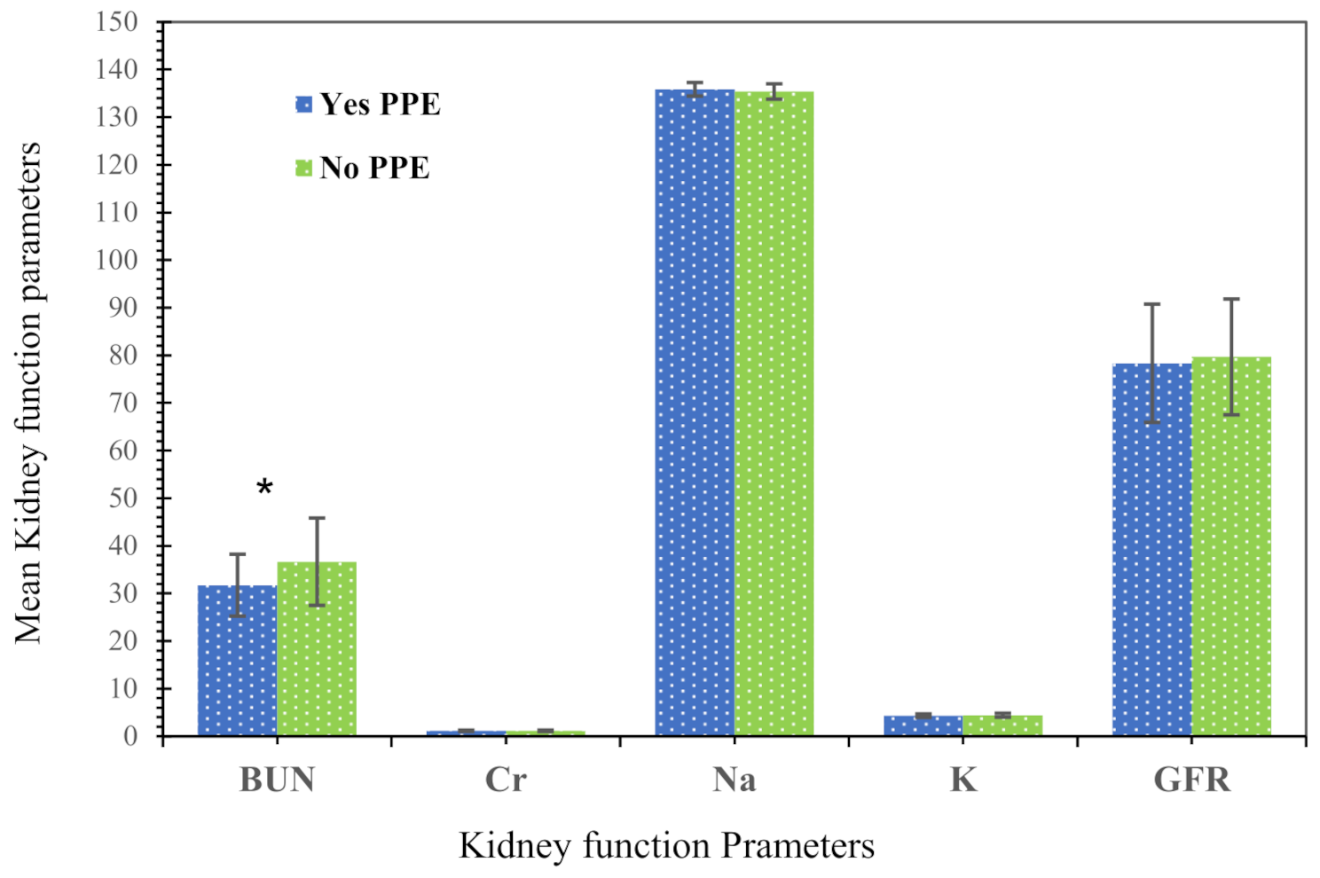
Participants’ information, including demographic characteristics, history of drug and supplement use, and disease history, was recorded in the researcher’s checklist. A pesticide exposure checklist [27] was completed, and laboratory examinations were performed on the participants. Kidney function was evaluated through laboratory indicators such as BUN and Cr [28, 29]. Blood samples were collected from each group in order to measure levels of blood urea nitrogen (BUN), creatinine (Cr), and electrolytes (sodium (Na), and potassium (K)) using spectrophotometry and an autoanalyzer. The glomerular filtration rate (GFR) was calculated using the Cockcroft-Gault formula. The most common measure of kidney activity was calculated using the Cockcroft-Gault formula: GFR = (140 − age) ×weight​/ plasma creatinine×72 × (0.85 in women) [30].

For the study, 5 ml of venous blood was drawn from each participant and placed in tubes without anticoagulant for BUN, Cr, Na, and K measurements. The samples were transferred to the laboratory within two hours, centrifuged, with the serum separated and stored at -70 degrees Celsius. The levels of BUN, Cr, Na, and K were then measured using spectrophotometry (Spect GENESYS 20) and an autoanalyzer (DIRUI, CS-400, China) according to the manufacturer’s instructions.

To examine pesticide exposure, several factors were considered: the processes of transportation, mixing, using pesticides, as well as repairing or cleaning spraying equipment. Exposure levels were influenced by the type of activity (e.g., using poisons, mixing), method of use (e.g., backpack sprayer, hand sprayer, speed sprayer), usage of personal protective equipment (PPE) (PPE such as gloves, masks, boots, clothing), along with work habits and personal hygiene practices (e.g., changing clothes or bathing after work). The intensity of pesticide exposure was calculated as follows:

Intensity of exposure to pesticides = (mixing mode + method of use + equipment repair or container washing) ×use of PPE.

The mixing mode was categorized into three levels: Never mixing was represented by a value of 0, less than 50% of mixing time involved was denoted by a value of 3 and, greater than 50% of mixing time involved was assigned a value of 9. The application method comprised seven levels: No spraying corresponding to a value of 0, aerial application and tablet distribution both represented by a value of 1, hole application valued at 2, tractor application assigned a value of 3, backpack application corresponding to a value of 8 and, hand spray application assigned a value of 9. The status of equipment repair or washing was a two-level variable: No repair or washing represented by 0 and equipment repair or washing corresponding to a value of 2.

There were four groups for Personal Protective Equipment (PPE) use, categorized as follows: PPE-0: 0% protection, no PPE used, PPE-1: 20% protection, (one of the following is observed: Face shield or glasses, Leather or cloth gloves, and boots), PPE-2: 30% protection, (one of the following is used: Special respirator, disposable clothing), PPE-3: 40% protection, special rubber gloves resistant to chemicals used. The PPE usage variable had eight levels: 1 = PPE-0, 0.8 = PPE-1, 0.7 = PPE-2, 0.6 = PPE-3, simultaneous use of: 0.5 = PPE-2 and PPE-1, 0.4 = PPE-3 and PPE-1, 0.3 = PPE-3 and PPE-2, and 0.1 = PPE-4 (combined protection of PPE-3 and PPE-2).

The monthly pesticide exposure index was determined by:

Monthly pesticide exposure index = years of spraying× number of days spraying per year​/30 days.

The cumulative exposure index was calculated as:

Cumulative exposure index = intensity of exposure×years of spraying×number of days spraying per year [31, 32].

Data were analyzed using SPSS version 22 software. Quantitative data were presented as mean ± standard deviation. The normality of quantitative variable distributions was first ascertained. Next, one-way analysis of variance (ANOVA) and either the chi-square test or Fisher’s exact test were employed to assess the homogeneity of the three groups regarding confounding variables.

Given the lack of age homogeneity among the groups, MANOVA was employed to compare other quantitative variables and to adjust for the effect of age. The assumptions of MANOVA, including the homogeneity of variances of dependent variables across groups, were evaluated using Levene’s test. Relationships between two quantitative variables were analyzed using Pearson’s correlation coefficient when parametric assumptions were fulfilled, or Spearman’s correlation coefficient when they were not. The significance level for all statistical tests was set at 0.05.