2.1 Data

Data were sourced from a randomised controlled trial conducted in Auckland and Christchurch, New Zealand (NZ) [20]. These data are termed the ‘NZ Gout Study’ herein. The study enrolled 200 participants with gout who were commencing allopurinol therapy. Participants were randomised 1:1 to receive colchicine 0.5 mg daily or placebo for 6 months. Colchicine plasma concentrations were measured in 80 participants at month 3 just prior to the daily dose and 30–60 min after the dose [20]. The study received ethical approval from the NZ Health and Disability Ethics Committee (18/STH/156). Participants provided written informed consent.

Samples from the NZ Gout Study were excluded if the dates and/or times of the colchicine measurement were missing. Missing independent variables such as covariates were inferred from the last observation unless the participant was missing all information about the covariate, in which case the participant was excluded. Samples below the lower limit of quantitation (LLOQ) for colchicine were excluded unless > 5% of the total samples were LLOQ, in which case a likelihood-based method [21] was explored.

Additional colchicine plasma concentration data were obtained for 13 individuals (ten healthy volunteers, one person with liver disease, one with gout and one with kidney disease) from published studies [5, 7, 10]. In these studies, data arose from the administration of single intravenous doses of 0.5 mg and 2 mg colchicine and 0.5-mg, 1-mg and 2-mg single doses of oral colchicine. Data points were extracted from published plasma concentration–time curves using PlotDigitizer Pro (v3.3.9, 2024). The extracted data were deemed necessary to provide structural model stability given the scant sampling in the NZ Gout Study.

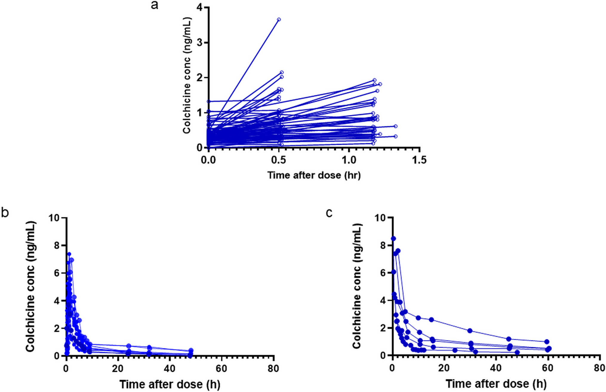
Observed colchicine plasma concentration–time plots from the NZ Gout Study and the extracted concentrations are presented in Fig. 1.

Fig. 1

Observed colchicine plasma concentration data used in the pharmacometric analysis. a The NZ Gout Study, b oral extracted data from the literature and c intravenous extracted data from the literature. Conc concentration, NZ New Zealand

2.2 Model Development

A population pharmacokinetic analysis was conducted using a non-linear mixed effects methodology in NONMEM (v7.5.1 ICON) and the first-order conditional estimation with interaction (FOCEI). The computer used a Windows 11 operating system, a 13th-generation Intel ® i5-1345U processor and a GNU Fortran 95 compiler. Workflow was managed using Pirana workbench (Certara, v23.10.1), and NONMEM was executed with Pearl—speaks NONMEM (PsN, v5.4.0). Pre- and post-processing used Prism v10.4.0 (GraphPad Software, La Jolla, CA), R v4.4.1 (The R Foundation) and MATLAB v2023b (MathWorks Inc.).

A published two-compartment pharmacokinetic model for colchicine with zero-order absorption and a time lag between the dose and systemic absorption (tlag) [22] was used as the starting point for base model development. This is termed the Karatze model. Details of the Karatze model parameter estimates are provided in the Electronic Supplementary Information (see Table S1 ). The Karatze model was parameterised in terms of clearance and volume for the central compartment, but the intercompartmental pharmacokinetics were parametrised as rate constants (\(_\) = 0.22 h−1 and \(_\)= 0.073 h−1) [22]. These were converted to intercompartmental clearance (\(Q\)) and peripheral volume (\(_)\) prior to model development as follows:

where \(_\) is the rate constant describing mass transfer from the central volume to the peripheral compartment, \(_\) is the central compartment volume and \(_\) is the rate constant describing mass transfer from the peripheral compartment to the central compartment. The Karatze model reported inter-individual variability in parameter estimates as standard deviations, as per the original publication from Thomas et al. [5]. These were converted to variances for the purposes of model building by squaring each value.

Model development followed a stepwise approach. First, a model was fit to the extracted intravenous data. Then, the oral extracted data were incorporated into the analysis and the parameters re-estimated. At this stage, oral availability (F) was estimated using a 'route' (RTE) parameter as follows:

$$\text=1 \, \left(\text\right)$$

$$\text=1+ _}\left(\text\right)$$

where \(F1\) is the oral availability for compartment 1 (gut), \(RTE\) is a multiplier for the route of administration and \(_\) is the estimated oral availability. The intention was to fix the estimate of F1 in subsequent modelling.

In the final modelling step, the colchicine data collected from 80 patients from the NZ Gout Study were incorporated into the analysis and the best model fit for the combined data (gout patients and extracted) explored. A parameter to account for the different tablet formulations used across studies was tested on bioavailability (F1). Differences in analytical methods between studies were explored.

While the Karatze model was used as a starting point, one- and two-compartment models were also explored, as well as first- and zero-order absorption with and without a time lag (tlag). Covariance was tested between all clearance and volume terms. Residual error was tested using additive, proportional and combined structures, while between-subject parameter variability was modelled using a log-normal distribution:

where \(_\) is the estimate of the \(^\) parameter \(\theta\) for the \(^\) individual, \(}_\) is the population mean value of the \(^\) parameter and \(_\) is the deviation from the mode of the \(^\) parameter for the \(^\) individual. \(\eta\) was assumed to be normally distributed with a mean of zero and a variance of \(^\).

Covariates to be tested in the model were selected based on visual inspection of exploratory data plots, biological plausibility and the availability of demographic and clinical data. Body size measures included total body weight (TBW), fat free mass (FFM) and normal fat mass (NFM). FFM was calculated using the formula developed by Janmahasatian et al. [23]. NFM followed the method outlined by Anderson and Holford [24, 25]. These metrics were standardised to 70 kg and allometrically scaled to a fixed exponent of ¾ for clearance parameters and to an exponent of 1 for volume parameters. A power model for body size with an estimated exponent was also tested on clearance. Creatinine clearance (CLcr) was estimated using the Cockcroft-Gault equation [26], standardised to 6 L/h/70 kg (approximately 100 mL/min/70 kg). CLcr was tested on CL/F using linear and power models as well as a model including both renal and non-renal clearance.

The influence of discrete covariates, including concomitant drugs, sex and ethnicity, was modelled using a fractional effect parameter. Ethnicity was self-reported in the gout study and included four categories: Māori, Pacific Peoples, NZ European and Other. Concomitant drugs included diuretics, statins, angiotensin receptor blockers (ARBs), angiotensin-converting enzyme inhibitors (ACEIs), alpha-blockers, beta-blockers and calcium channel blockers (mostly dihydropyridines). Drugs known to be strong or moderate CYP3A4 or P-glycoprotein inhibitors based on the Flockhart Table [27] and UpToDate [28] were grouped together and tested for a fractional effect on colchicine clearance. The same analysis was repeated for strong or moderate CYP3A4 or P-glycoprotein inducers, including the use of prednisone for gout in the weeks prior to the clinical visit at month 3. Age and adherence (based on measured pill counts at month 3) were tested using linear models as well as a fractional effect based on binned categories.

2.3 Model Building and Evaluation

Decisions about best model fit to the data were based on a likelihood ratio test, parameter precision, the plausibility of parameter estimates, visual inspection of goodness-of-fit plots and prediction-corrected visual predictive checks (pcVPCs). For the likelihood ratio test, a decrease in the objective function value (OFV) of 3.84 units (Chi-square [\(^\)], p < 0.05) with 1 degree of freedom was considered statistically significant.

A base model was first developed to determine the best structural model and the statistical components including random residual variability and between-subject variability. Subsequent covariate modelling followed a stepwise method. Each covariate was tested in the final base model one at a time using a likelihood ratio test. Only those covariates found to produce a better statistical fit to the data were retained for the next step. In step 2, the covariate that produced the biggest univariate drop in OFV was retained in the model and each of the remaining covariates tested one at a time. In step 3, the two covariates that produced significantly better model fit in steps 1 and 2 were retained and the remaining covariates added again one at a time. This was repeated until all significant covariate relationships had been identified. The full model was subjected to backwards elimination of each covariate, and only those that resulted in an increase in the OFV of > 6.6 units (χ2, p < 0.001) with 1 degree of freedom on removal were retained in the final model.

pcVPCs were derived by simulating 100 data sets using the final colchicine pharmacokinetic model and plotting the 5th, 50th and 95th percentiles of the model predictions against the same percentiles of the observed data. pcVPCs were stratified by study, route of administration and for any significant covariates. The median parameter values and the 95% confidence intervals (CIs) were determined from 2000 replicates using a sampling-importance-resampling method (SIRSAMPLE in NONMEM) where replicate parameter values were derived from importance sampling [29]. This method was used in lieu of a nonparametric bootstrap to handle the unbalanced study designs described here [29].

2.4 Colchicine Plasma Concentration Predictions

Steady-state colchicine plasma concentrations were predicted from the final population pharmacokinetic model in MATLAB (v2024b). A series of stochastic simulations under dosages of 0.5 mg, 1 mg and 1.5 mg once or twice daily and under different covariate conditions were conducted. For each scenario, n = 1000 stochastic profiles were generated for a 40-day colchicine treatment period. The steady-state plasma concentrations across a 24-h period on day 40 were used to generate the following steady-state exposure metrics for each simulate:

1.

Cmin,ss: the concentration just prior to the dose.

2.

Cmax,ss: the maximum concentration after the dose.

3.

Cav,ss: the steady-state average plasma concentration.

The percentage of values below and above the proposed therapeutic range of 0.5–3 ng/mL was determined. For the purposes of these analyses, we considered colchicine doses that produced > 80% of steady-state average concentrations < 3 ng/mL and > 0.5 ng/mL to have a reasonable probability of safety and efficacy. Note that the steady-state average concentration was chosen under the assumption that transient Cmin,ss or Cmax,ss concentrations below or above the limits of therapeutic range across a dosing interval may not appreciably impact safety and efficiency.

Covariates were sampled as a group from a dataset of virtual people with gout. The methodology used to create the virtual datafile is described in the Electronic Supplementary Information, including the MATLAB code. A comparison of patient characteristics in the observed and virtual datasets is presented in Table S2. Each simulate was randomly assigned a set of patient characteristics including all factors found to be significant in the covariate modelling.