2.1 Study Population2.1.1 Included Clinical Studies

This population modeling analysis included FIX activity data of participants with hemophilia B from a total of 11 clinical trials (Table S1, see electronic supplementary material [ESM]). Data were pooled from eight studies of nonacog alfa [22] (BeneFIX®, an SHL recombinant FIX replacement therapy; n = 274 participants) and three studies of fidanacogene elaparvovec (n = 63 participants). Participants in the fidanacogene elaparvovec studies received a one-time dose of the gene therapy and on-demand doses of a range of SHL or EHL FIX replacement therapies (Table S2, see ESM).

2.1.2 Study Assessments

FIX activity in plasma samples was analyzed with a one-stage clotting assay for each study. In the nonacog alfa studies, plasma samples were analyzed by a validated activated partial thromboplastin time (aPTT)-based method using a multi-channel discrete analyzer. In the fidanacogene elaparvovec studies, plasma samples were analyzed using an Actin® FSL reagent and BCS® XP analyzer (validated at Colorado Coagulation/Esoterix Lab Services [Englewood, CO, USA]). Descriptions of FIX activity sampling times per study protocol and the limits of quantification for the one-stage clotting assays are provided in Table S1 (see ESM).

2.1.3 Exclusion Criteria and Missing Data

Participants who did not receive at least one dose of fidanacogene elaparvovec or FIX replacement therapy or did not have at least one FIX activity measurement (with correct dosing and time information) were excluded from this analysis. Below limit of quantification (BLQ) observations were considered as missing and were excluded during estimation of population parameters.

2.2 Population Modeling Analysis2.2.1 Software

Nonlinear mixed-effects modeling was implemented using NONMEM® version VII level 5.0 (ICON Development Solutions, Ellicott City, MD, USA) [23]. Population parameter estimates used a first-order conditional estimation method with interaction. Individual parameters were obtained from empirical Bayes estimates (EBEs). The ADVAN13 subroutine with TOL = 9 was used for solving differential equations. Perl-speaks-NONMEM 5.2.6 was used for sampling importance resampling (SIR). Statistical and graphical outputs were generated using the R programming and statistical language [24].

2.2.2 Structural Model Development

A structural model was developed to describe FIX activity following administration of nonacog alfa and/or fidanacogene elaparvovec. The model aimed to incorporate all contributing endogenous and exogenous sources of FIX activity. As such, a model of gene and protein expression dynamics (Hargrove-Schmidt) [25] was extended using nonlinear mixed-effects modeling to describe the disposition of FIX activity from all sources.

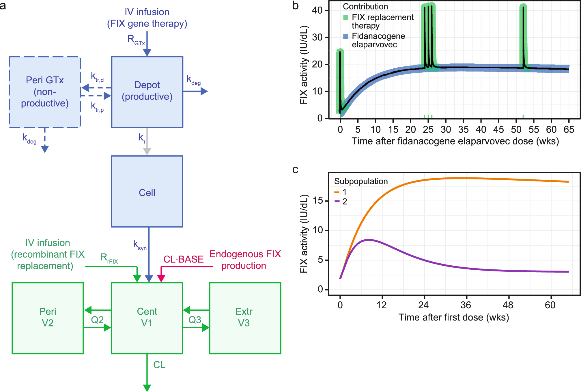
The two-compartment Hargrove-Schmidt model describes translation of transgene-produced FIX protein by a first-order process as a function of the total number of vector genomes administered (i.e., the gene therapy dose). Importantly, there is no loss of transgene from the compartment upon translation to FIX protein. Instead, transgene loss or degradation is described by a separate first-order rate constant. This framework was extended to account for disposition of FIX following endogenous FIX production, secretion of transgene-derived FIX into the plasma, and administration of SHL or EHL FIX replacement therapy (see Fig. 1a).

Fig. 1

Schematic of final structural model and model’s description of FIX activity. a Schematic of the final structural model (including FIX synthesis, transgene degradation, and FIX disposition and elimination). Colors indicate the components describing the contribution of fidanacogene elaparvovec (blue), SHL/EHL FIX replacement therapy (green), or endogenous FIX (red) to model-predicted FIX activity. \(__}\) zero-order infusion rate of fidanacogene elaparvovec (vg/h), \(DEPOT\) amount of productive transgene (vg), \(_\) amount of non-productive transgene for subpopulation 2 (vg), \(CELL\) amount of FIX in the site of FIX synthesis (IU), \(_\) first-order rate constant for degradation of transgene (h−1), ktr,d first-order rate constant for transgene transition from the productive to non-productive state (h−1), \(_\) first-order rate constant for transgene transition from non-productive to productive state (h−1), \(_\) first-order rate constant for turnover of FIX at the site of action (h−1), \(_\) translation constant for the ratio of gene to expressed protein (IU/vg h−1), \(BASE\) baseline FIX activity (IU/dL), \(_\) zero-order infusion rate of rFIX replacement (IU/h), \(CENT\) and \(V1\) amount of FIX in and volume of the central compartment (IU and dL, respectively), \(PERI\) and \(V2\) amount of FIX in and volume of a potential peripheral compartment (IU and dL, respectively), \(EXTR\) and \(V3\) amount of FIX in and volume of a potential extravascular compartment (IU and dL, respectively), \(CL\) clearance from the central compartment (dL/h), \(Q2\) inter-compartmental clearance between the central and peripheral compartments (dL/h), \(Q3\) inter-compartmental clearance between the central and extravascular compartments (dL/h). b Final model’s description of the contributions of fidanacogene elaparvovec and FIX replacement therapy to overall FIX activity. Dosing scenario is an example for demonstration purposes and is not representative of a specific study individual. The black line is the population-typical model-predicted FIX activity for an individual with body weight 86.1 kg administered 5 × 1011 vg/kg of fidanacogene elaparvovec and five doses of SHL FIX replacement therapy 40 IU/kg at Weeks 0, 24, 25, 26, and 52. The blue and green shaded areas represent the contributions of fidanacogene elaparvovec and SHL FIX replacement therapy to the predicted FIX activity as described by the model. Green indicators on the x-axis are the times when SHL FIX replacement therapy was administered. c Final model’s description of FIX activity for different population phenotypes (constant FIX production [subpopulation 1], transient FIX production [subpopulation 2]). Solid lines represent the FIX activity (as assessed by Actin® FSL assay) time-course for a population-typical individual (weight 86.1 kg, aged 35 years, manufacturing process 3) administered 5×1011 vg/kg of fidanacogene elaparvovec as described by the phenotype for subpopulation 1 (orange) or subpopulation 2 (purple). EHL extended half-life, FIX factor IX, SHL standard half-life

The model was built from combined data from nonacog alfa and fidanacogene elaparvovec studies in a two-stage process. Data from nonacog alfa studies were used to develop a structural model that quantitatively described FIX disposition and clearance. One-, two-, and three-compartment models were tested to describe FIX disposition, with parameters for clearance (\(CL\)), volume of distribution of compartment 1 (\(V1\)), volume of distribution of compartment 2 (\(V2\)), volume of distribution of compartment 3 (\(V3\)), inter-compartmental clearance between compartment 1 and 2 (\(Q2\)), and inter-compartmental clearance between compartment 1 and 3 (\(Q3\)). The model included a parameter for baseline FIX activity (\(BASE\)) resulting from endogenous FIX production or inadequate washout of prior FIX replacement therapy.

Data from fidanacogene elaparvovec studies were pooled with the nonacog alfa studies to describe FIX synthesis and transgene degradation. Parameters accounting for gene and protein expression dynamics included a translation constant for the ratio of transgene to FIX protein (\(_\)), a first-order rate constant for turnover of FIX at the site of action (\(_}\)), and a first-order rate constant for degradation of the transgene (\(_}\)).

The effects of body weight were included a priori for all clearances, volumes, and first-order rate constants via allometric scaling (referenced to a 70-kg individual) with fixed exponents of 0.75, 1, and − 0.25, respectively [26].

Participants in the gene therapy trials received a single dose of fidanacogene elaparvovec; therefore, the model was not intended to address re-administration. The fidanacogene elaparvovec dose was calculated based on the release titer for the product lot and input into the population model. Participants in the fidanacogene elaparvovec trials could also receive FIX replacement therapy during the study (on-demand or resumption of prophylaxis if FIX activity was ≤ 2 IU/dL or spontaneous bleeds reoccurred). The model accounted for the contributions of any FIX replacement therapy dose on FIX activity. Table S2 summarizes the FIX replacement therapy products administered in the fidanacogene elaparvovec trials and the population PK models used to account for their administration (see ESM).

Predicted FIX activity from all endogenous and exogenous sources was calculated as

where \(_\) is the model-predicted FIX activity in individual, \(i\), at observation, \(j\), \(FIXA\) is an estimable parameter quantifying the relative differences in FIX activity between different data sources, \(_/_\) is FIX activity in the central compartment from combined SHL FIX products (nonacog alfa and plasma-derived FIX) and fidanacogene elaparvovec, and \(_\) is the FIX activity contribution from EHL products.

For random effect parameters, inter-individual variability (IIV) was assumed to be log-normally distributed:

where \(_\) is the individual value for parameter, \(P\), in the ith individual, \(_\) is the population typical value for parameter \(P\), and \(_\) is an independent random variable describing the variability in \(P\) among subjects with a mean of 0 and variance, \(^\).

Random unexplained variability (RUV) in FIX activity was described by an additive residual error model (in the log domain):

$$log\left(_\right)=log\left(_\right)+_}$$

where \(_\) is the FIX activity in individual, \(i\), at observation \(j\), \(_\) is the model predicted FIX activity, and \(_}\) is a normally distributed error term with means of 0 and variances of \(_}^\).

The addition of fixed effect parameters was evaluated based on the Akaike information criterion (AIC) for non-hierarchical models. Models with lower AIC values (i.e., a decrease in AIC by more than two units with the addition of one estimable parameter) were ranked higher for model selection.

2.2.3 Covariate Model Development

A stepwise covariate modeling approach was used to assess potential predictors of variability in gene-therapy parameters. Selection of potential covariates was based on mechanistic, physiological, and clinical plausibility. Screened covariates (assessed on key population parameters) included age (effect on \(CL\), \(_}\), \(_}\), \(_\), \(BASE\), \(FIXA\), and the log-odds of being assigned to a subpopulation parameter), manufacturing process (effect on \(_}\), \(_}\), \(_\)), concomitant steroids (yes/no effect on \(_}\), \(_}\), \(_\), and mixture model parameters), body weight (effect on \(_\)), and body mass index (BMI) (effect on \(_\)).

Categorical covariate effects were represented as a discrete relationship (e.g., the effect of manufacturing process, \(CSGRPN\), on a parameter, \(P\)):

$$_=_ \cdot ^_} \cdot PCSGRPN\begin& for& \endPCSGRPN=\left\1\\ 1\\ 1\\ 1\end\right.\begin\\ +\,__}\\ +\,__}\\ +\,__}\end \begin\text=0\\ \text\text=1\\ \text=2\\ \text\end$$

where \(_\) is the individual value for parameter, \(P\), in the ith subject, \(_\) is the population-typical value for parameter \(P\), \(CSGRPN\) has a value of 0 for observations not associated with fidanacogene elaparvovec therapy, 1 for process 1, 2 for process 2, and 3 for process 3, and \(__,3}}\) are estimable parameters for the effects of manufacturing processes on \(P\).

Continuous covariate effects were represented as a power function referenced to the median of observed data (e.g., the effect of age on a parameter, \(P\)):

$$_=_ \cdot ^_} \cdot \left(\frac_}_}}\right)}^_}$$

where \(_\) is the age (years) in the ith individual, \(_}\) is the median age in the observed population, and \(_\) is an estimable parameter for the effect of age on \(P\).

Covariates were screened for pairwise correlations via graphical analysis. If covariates were strongly correlated (r < − 0.7 or r > 0.7), the more clinically relevant covariate was selected for further analysis. The relationship of covariates to variability in parameters was assessed with plots of individual EBEs of model parameters versus candidate covariates (scatterplots with linear-regression trend lines or box-and-whisker plots for continuous and categorical covariates, respectively).

Candidate covariates were independently added to the final structural model, and their individual significances in improving model fit were assessed by likelihood ratio test (LRT; significance level, p < 0.01). Candidate covariates also had to meet additional necessary criteria: the 95% confidence interval (CI) of the parameter estimate did not include zero (no effect), the addition of the covariate resulted in a reduction in IIV on the target population parameter (if applicable), and model diagnostic plots showed improvement. All covariates identified as significant in univariate analyses were carried forward to multivariate analysis and added sequentially to the prior final model in order of statistical significance. The sequential addition of a covariate to the model needed to satisfy all requirements described for univariate analyses.

2.2.4 Model Assessments

Perceived outlier observations (absolute conditional weighted residuals [CWRES] > 6) were not considered for removal because of the possibility that they could be due to unaccounted doses of FIX replacement therapy or transient changes in FIX activity. Model adequacy was assessed by changes in the minimum objective function value (OFV) and condition number (square root of the ratio of the highest and lowest eigenvalues). Models with condition numbers < 100 were highly considered [27].

Model performance was assessed with diagnostic plots including (i) observed concentrations versus population predictions (PRED) or individual predictions (IPRED), (ii) CWRES versus time after first dose or PRED, (iii) distribution density and quantile-quantile plots to evaluate the normality of CWRES distributions, (iv) distribution density plots to evaluate the normality of \(\eta\) distributions (as described by individual EBEs for random effect parameters), and (v) individual predicted concentration–time profiles overlaid with observations.

SIR was used to obtain the median and 95% CI of parameter estimates [28]. Five iterations of sampling (1000, 1000, 1000, 2000, and 2000) and re-sampling (200, 400, 500, 1000, and 1000) were conducted. The proposal distribution was derived from the multivariate variance-covariance matrix of parameter estimates from the final model. Resamples served as the proposal distribution for the subsequent iteration. The 95% CIs of final parameter estimates were constructed from 1000 samples of the final iteration. The predictive performance of the final model was evaluated by a visual predictive check (VPC) and a prediction-corrected VPC [29].

2.3 Model-Based Simulations

Simulations were performed with a virtual population of 100,000 individuals with hemophilia B. Parameters were randomly drawn from IIV distributions as described by the final model. Required demographic characteristics were randomly sampled from distributions representative of the adult analysis populations from the combined clinical studies. FIX activity was predicted for up to 15 years for each simulated individual following administration of fidanacogene elaparvovec (nominal dose: 5 × 1011 vector genomes per kilogram of body weight [vg/kg], using the commercial manufacturing process [process 3]). The median and 90% prediction intervals (PIs) were calculated for the following summary metrics: FIX activity over time; peak FIX activity; time to peak FIX activity; area under the curve for the follow-up interval (i.e., 15 years; \(}_\)); time to 50, 60, 70, 80, 90, 95, and 99% of peak FIX activity; and time within 50, 60, 70, 80, 90, 95, and 99% of peak FIX activity.