2.1 Imaginary Effects of Top Neutral Indicators

In Appendix (A.3) an estimate of the average correlation coefficient with the phenotype (by modulus) is obtained for k top neutral predictors:

$$_} = \fracE\left( = m - k + 1}^m \left| _},Y} \right)} \right|} \right),$$

where the sum is taken from k top neutral variables Xi selected from m studied.

The average value of the correlation module for independent Gaussian features is

$$E\left| _},Y} \right)} \right| = \sqrt }} .$$

However, the top values at m \( \gg \) n > k may be significantly higher. In the theory of order statistics, there are results describing the distribution of the sum of k top values [14]. With their help, the following estimate was obtained in Appendix A.3 for r0 at m \( \gg \) k:

$$_} = \sqrt }\frac^}}}^}}}} ,$$

(4)

where n is the sample size, m is the number of neutral predictors studied, and k is the number of top predictors by effect used to construct multiple regression. Thus, random correlations of the phenotype with top neutral predictors are proportional \(\sqrt } \) and, as expected, are inversely proportional \(\sqrt n \).

2.2 The Coefficient of Determination for the Regression Constructed on the Top Neutral Variables

Using formulas (3) and (4), one can obtain an estimate of the coefficient of determination \(R_^\) determined exclusively by neutral top predictors. Assuming that, for all top neutral predictors approximately \(r_^ \approx r_^\), from Eq. (3) we have

$$R_^ = \frac^}} \right)r_^}} = \frac}\frac^}}}^}}}}} \right)}\frac^}}}^}}}}}.$$

(5)

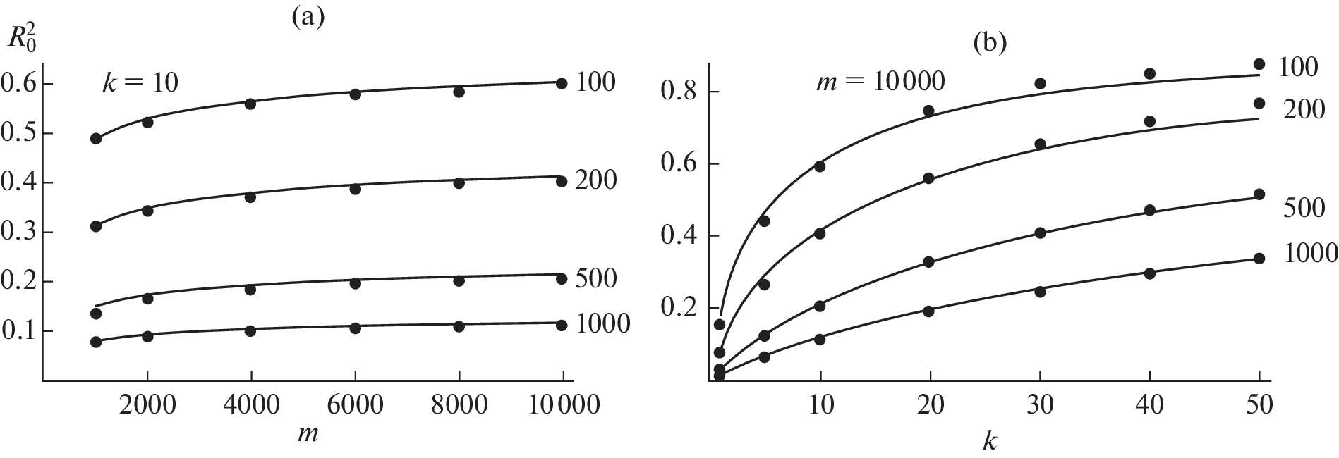
This is the desired estimate of the coefficient of determination under the null hypothesis that all top predictors are neutral, i.e., not associated with the phenotype Y. Figure 1 demonstrates the correspondence of formula (5) to the estimates obtained in computer simulations.

Fig. 1.

Dependence of the coefficient of determination under the null hypothesis (\(R_^\)) on the number of studied (m) and the number of selected top predictors (k) for different sample sizes (n). The solid lines are estimates using formula (5). The dots are the average results of computer simulations for 500 repetitions. (a) Dependence of \(R_^\) on m at k = 10; (b) dependence of \(R_^\) on k at m = 10 000.

2.3 Reproducibility of Effects in Test Samples

By reproducibility of regressions, we mean the ratio \(}}}^} \mathord}}}^} ^}}}} \right. \kern-0em} ^}}}\), where R2 is the square of the multiple correlation for the discovery sample and \(R_}}}^\) is the square of the one-dimensional correlation of the phenotype Y with a forecast for the test sample. The forecast is made using the regression equation obtained for the opening sample. To study the question of reproducibility of effects, it is necessary to postulate that some of the predictors Xi are causally related to the phenotype Y. We will do this in the simplest way, assuming that, from m predictors, only m1 have an additive effect on Y:

$$Y = _} + _} + ... + __}}}} + \varepsilon .$$

We assume the same mechanism of formation of phenotype Y in the training and test samples. It is hardly possible to obtain analytical expressions for correlations in the training sample and the test sample, even in the case of independent predictors. Therefore, in the following, to assess the reproducibility of effects in test samples, we will limit ourselves exclusively to computer simulations.

Computer simulations show a surprising pattern: over a wide range of values n, m, m1, and k, the reproducibility of regressions depends primarily on the ratio \(^} \mathord^} ^}}}} \right. \kern-0em} ^}}}\) in the discovery sample. This is demonstrated in Fig. 2, which shows the dependence \(}}}^} \mathord}}}^} ^}}}} \right. \kern-0em} ^}}}\) on \(^} \mathord^} ^}}}} \right. \kern-0em} ^}}}\) for different values of m and m1. Variation of values of \(^} \mathord^} ^}}}} \right. \kern-0em} ^}}}\) at fixed m and m1 was carried out by changing the value of n in the range from 100 to 2000. The number of top predictors was chosen equal to k = m1. The points were obtained by averaging 500 repetitions.

Fig. 2.

Dependence of reproducibility (ratio \(}}}^} \mathord}}}^} ^}}}} \right. \kern-0em} ^}}}\)) on the relationship \(^} \mathord^} ^}}}} \right. \kern-0em} ^}}}\) at different values of n, m, and k. Here \(R_^\) is the null hypothesis, R2 is the training sample, and \(R_}}}^\) is the independent test sample. The points are obtained by averaging 500 repetitions. The point (0.75, 0.5) is marked, where half of the original coefficient of determination is expected in the test sample.

From Fig. 2, it is clear that, if \(^} \mathord^} ^}}}} \right. \kern-0em} ^}}}\) < 0.75, then more than half of the original coefficient of determination can be expected in the test sample.

2.4 Prediction of Reproducibility by Maximum Correlation in the Discovery Sample

It is even easier to control the reproducibility of effects through the maximum absolute value of the correlation coefficient in the discovery sample. The mathematical expectation of the maximum correlation in the case of neutral features (\(r_}^}\)) can be estimated using formula (4), substituting there k = 1:

$$r_}}}^} = \sqrt }\frac^}}}} .$$

This is an estimate of the correlation coefficient of the phenotype with the top neutral predictor, i.e., under the null hypothesis that all predictors are not associated with the phenotype. Let rmax = \(\mathop \limits_i Cor(Y,_})\) be the maximum absolute value of the correlation coefficient in the presence of causal predictors. Then, comparing rmax with the magnitude of \(r_}^}\), one can judge the reproducibility of effects in test samples. This is shown in Fig. 3, which shows the dependence of reproducibility on the ratio \(}^}} \mathord}^}} _}}}}} \right. \kern-0em} _}}}}\) for different values m and m1. Variation of values of \(}^}} \mathord}^}} _}}}}} \right. \kern-0em} _}}}}\) at fixed m and m1 was carried out by changing the value n in the range from 100 to 2000. The number of top features was chosen equal to k = m1. The points were obtained by averaging 500 repetitions.

Fig. 3.

Dependence of reproducibility (ratio \(}}}^} \mathord}}}^} ^}}}} \right. \kern-0em} ^}}}\)) on the relationship \(}^}} \mathord}^}} _}}}}} \right. \kern-0em} _}}}}\) at different values n, m, and m1. Here \(r_}^}\) is the maximum correlation at m neutral predictors, and rmax is the maximum correlation for the training sample at m1 causal predictors. The points are obtained by averaging 500 repetitions. The point (0.8, 0.5) is marked, where half of the original coefficient of determination is expected in the test sample.

From Fig. 3, it is clear that, if \(}^}} \mathord}^}} _}}}}} \right. \kern-0em} _}}}}\) < 0.8, then more than half of the original coefficient of determination can be expected in the test sample. At \(}^}} \mathord}^}} _}}}}} \right. \kern-0em} _}}}}\) < 0.6, the reproducibility reaches 100%. Thus, to reliably reproduce the effects, it is necessary that the observed maximum correlation in the discovery sample exceed the calculated top correlation of the neutral feature by 1.25 times.

We believe that the observed patterns are of a fairly general nature, although we do not have a mathematical justification for this fact.

2.5 Achieving a “Genome-Wide Significance Level” Does Not Guarantee Reproducibility

In this section, we demonstrate that the passage of the indicator with the maximum effect through the Bonferroni threshold does not at all guarantee high reproducibility of the effect in test samples. This is especially noticeable when the number of predictors studied is very large. Table 1 shows the top predictors in terms of effect at m = 1 000 000 for two models: neutral and causal. For the neutral model, all predictors are unrelated to the phenotype; in the causal model, there are 50 predictors that influence the phenotype. From Table 1, it is evident that, with the sample size n = 600, the top indicator overcomes the Bonferroni threshold (p < 5E-8), but the reproducibility in test samples is only 7%.

Table 1.   Top predictor in terms of effect at m = 1 000 000: a model with neutral predictors and a model in which 50 predictors are causal2.6 Practical Recommendations

The practical use of the presented methods is quite obvious. By comparing the actually observed multiple correlation with the estimate (5), we can judge the prospects for further research and the very possibility of constructing a PRS (polygenetic risk score) on the basis of data for the discovery sample. From Fig. 2, it is evident that high reproducibility is observed if the coefficient of determination in the training sample is 2–3 times higher than \(R_^\). In order for at least half of the original squared correlation to be observed in the test sample, it is necessary that, in the discovery sample, \(^} \mathord^} ^}}}} \right. \kern-0em} ^}}}\) < 0.75; i.e., the coefficient of determination in the discovery sample should be 1.3 times higher than \(R_^\) (see Fig. 2).

Comparison rmax with \(r_}^}\), i.e., the maximum observed correlation with the theoretically expected one for neutral predictors, is particularly useful when evaluating new publications of GWAS results. From GWAS summary statistics, it is usually easy to find the predictor with the top effect. If the correlation coefficient for this indicator exceeds \(r_}^}\) by more than 1.25 times, then we can expect confident reproduction of the effects in the test samples (point with coordinates (0.8, 0.5) in Fig. 3).

The author successfully uses these simple criteria in his own practice of statistical processing of primary GWAS and EWAS data (for example, [16]).

When planning pilot experiments, the significant role of the size of the training sample n should also be taken into account in the prospects for further use of the results obtained. At m = 1000, to achieve reproducibility, \(}}}^} \mathord}}}^} ^}}}} \right. \kern-0em} ^}}}\), more than 50%, a training sample size n = 200 is sufficient. To meet the same requirements at m = 500 000, the training sample size should be n > 400.