We assume that an uninterrupted drug dose (giving rise to constant drug levels) yields the following deterministic relationship for cell i

$$\begin k_i(t)=k_i(0)\exp (-\delta t), \end$$

(2)

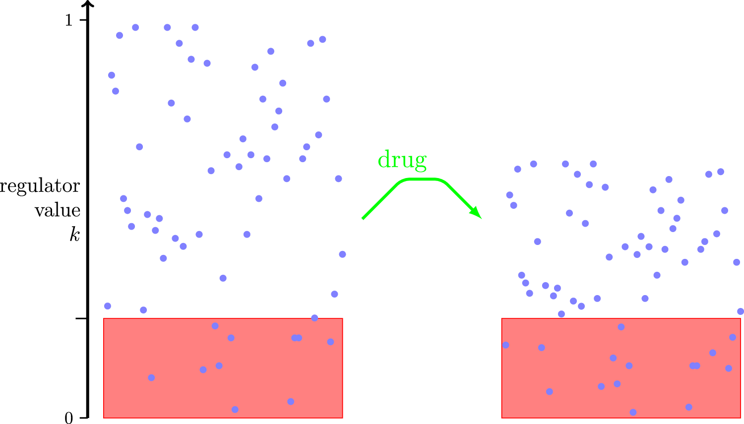
and that cells with \(k_i(t)<0.25\) are in the death pool. In the simplest case, the death rate of any cell in the death pool is equal to a constant \(\mu\). Cells with \(k_i(0)>0.25\) are not initially in the death pool but enter the pool when their regulator value has decreased to 0.25. Figure 2 is a small-scale illustration of the resulting dynamics: the ten cells initially present die, one by one, as their regulator values decline under the influence of the drug, taking them into the death pool.

Illustrating the effect of a sustained dose on a population of 10 cells. Each blue line is the regulator attribute of one cell as a function of time. Lines terminate in blue dots that indicate cell death. Cells are said to be in the death pool when their regulator value is less than 0.25, indicated by red shading. Simple model without cell division, with parameter values \(\delta =0.2\) and \(\mu =1\)

Let \(t_k\) be the first time that a cell, whose initial regulator value is equal to k, enters the death pool. The lifetime of the cell is the sum of \(t_k\) and the time to die once the cell enters the death pool. We can calculate \(t_k\) using (2):

$$\begin t_k = \inf \ \ = \ 0 & \qquad 0\le k \le \frac\\ \dfrac\log (4k) & \qquad \frac < k \le 1. \end\right. } \end$$

(3)

This time is shown on the LHS in Fig. 3. On the RHS, two possible functions w(k) are shown. We will use \(w_0(k)\) in this Section and \(w_1(k)\) in the Supplementary Material, where

$$\begin w_0(k)= 0 & k>\frac\\ \mu & k<\frac.\end\right. } \end$$

(4)

Left: The time, \(t_k\), at which a cell enters the death pool is shown as a function of the cell’s initial scaled regulator value. Right: two death-rate functions \(w_0(k)\) and \(w_1(k)\)

Consider a cell chosen at random from a population with initial regulator values uniformly distributed between 0 and 1. The probability that it survives to t is obtained by integrating (1):

$$\begin S(t) = \left( \text t\right) } = \int _0^1 s(t,k) \textrmk. \end$$

(5)

We evaluate the integral in (1) using (4) to yield the probability that a cell labelled i survives to time t:

$$\begin s(t,k) = \left( \text t|k_i(0)=k\right) }= 1 & \qquad t \le t_k\\ \textrm^& \qquad t>t_k. \end\right. } \end$$

(6)

Figure 4 shows s(t, k) as a function of t using four values of k (upper) and as a function of k using four values of t (lower).

Upper: s(t, k) is the probability that a cell, whose initial regulator value is k, is still alive at time t when \(w(k)=w_0(k)\). If k is fixed then s(t, k) is a non-increasing function of t. Lower: The probability that a cell, whose initial regulator value is k, is still alive. If t is fixed then s(t, k) is a non decreasing function of k. The formula used is (6), with \(\mu =1\) and \(\delta =0.5\)

Next, consider a cell chosen at random from a population with initial regulator values uniformly distributed between 0 and 1. The probability that a cell, chosen in this way, survives to t is found by evaluating the integral in (5) as follows:

$$\begin S(t)&= \frac\textrm^ +\int _}^1s(t,k)\textrmk\end$$

(7)

$$\begin&= \frac\textrm^ + \textrm^ \displaystyle \int _}^\textrm^} (4k)^\textrmk + 1-\frac\textrm^& \hspace\delta t<\log 4\\ \textrm^ \displaystyle \int _}^1 (4k)^ \textrmk& \hspace\delta t \ge \log 4. \end\right. } \end$$

(8)

Note that, if \(k>\frac\) then \(\textrm^ = (4k)^\). On the RHS in (8), the term \(\frac\textrm^\) corresponds to cells that are in the death pool at \(t=0\) (and remain there). The term \(1-\frac\textrm^\) is the fraction of cells that are not in the death pool. Evaluating the integrals,

$$\begin S(t) = 1- \dfrac\dfrac^-\textrm^} & \qquad \delta t \le \log 4\\ A\textrm^\qquad & \qquad \delta t \ge \log 4, \end\right. } \end$$

(9)

where

$$\begin A = \int _0^1\textrm^\textrmk = \dfrac+\frac\frac}}. \end$$

(10)

The factor A is an increasing function of the ratio \(\mu /\delta\), with \(A=1\) when \(\mu /\delta =0\). In the limit \(\mu /\delta \rightarrow 0\), the action of the drug is fast compared to the typical survival time of a cell in the death pool.

The probability density of single-cell death times, shown as the top panel in Fig. 6, is obtained from the derivative of S(t):

$$\begin f(t) = -S'(t) = \dfrac^-\mu ^2\textrm^} & \qquad \delta t \le \log 4\\ \mu A\textrm^\qquad & \qquad \delta t \ge \log 4. \end\right. } \end$$

(11)

The mean time to death of a single cell will be denoted \(\textrm\!\textrm(\tau _1)\). It is equal to the sum of the mean time to arrive in the death pool plus the mean time to die once in the death pool:

$$\begin \textrm\!\textrm(\tau _1) = \int _}^1t_k\textrmk + \frac = \frac(\log 4-\frac)+ \frac. \end$$

(12)

The variance of \(\tau _1\) is

$$\begin \text (\tau _1) = \dfrac. \end$$

(13)

Note that the variability of the mean time to death of a single cell is a function only of the time the cells take to die once they arrive in the death pool.

Suppose there are n tumour cells at \(t=0\), with regulator values uniformly distributed in (0, 1). How long until all n cells die? An example realisation, with \(n = 100\), calculated using the single sustained dose model described above, is shown in Fig. 5. That is, the blue line is a number of cells surviving to time t when each, independently, is assigned an initial regulator value in (0, 1) and, under the action of the drug, enters the death pool.

Blue: The number of surviving cells as a function of time in one realisation of the single, sustained dose model. Also shown is the smooth function obtained by averaging over many realisations, equal to the survival function S(t) (9) multiplied by the initial number of cells. The vertical dotted line indicates \(t=\log 4/\delta\). Here \(n=100\), \(\delta =1\) and \(\mu =0.2\) (Color figure online)

We define the random variable \(N_t\) to be the number of cells alive at time t, with \(N_0=n\). Let \(\tau _n\) be the first time that \(N_t=0\). Inspecting (9), we see that the single-cell survival probability has a simple exponential form as long as \(\delta t > \log 4\). The form is \(S(t)=A\textrm^\) is found if an individual lifetime is drawn as a random variable that is the sum of a fixed time of duration \(\log A/\mu\) and an exponentially-distributed time with mean \(1/\mu\). The time to extinction of n such individuals (\(\textrm\!\textrm(\tau _n)\)) is given by [21]

$$\begin \textrm\!\textrm(\tau _n) = \frac\left( \log A +1 + \frac+\frac+\cdots +\frac\right) \simeq \frac\left( \log nA + \gamma \right) , \end$$

(14)

where \(\gamma =0.577\ldots\). We use the symbol \(\simeq\) to denote the large-n approximation. Similarly [22, 23]

$$\begin \text (\tau _n) = \frac\left( 1+\frac+\frac+\cdots +\frac\right) \simeq \frac\frac. \end$$

(15)

Probability density of extinction times, sustained dose with \(n=1\), 10, 100 and 1000. Solid red lines are the exact formulae; the blue histograms are compiled from 10,000 numerical realisations. The same horizontal scale is used in each case, with \(\mu =0.2\) and \(\delta =1\). Top: \(n=1\). The maximum is at \(t=\frac\log 4\), after which all cells are in the death pool. In each of the lower three panels, the vertical dotted line is \(t_\textrm=\frac\log (nA)\). The ratio \(\mu /\delta\) determines the factor A

As can be seen in Figs. 5 and 6, a considerable simplification arises because typical values of \(\tau _n\) are large compared to \(1/\delta\). When \(\delta t>\log 4\), \(\left( \text t\right) }=1-A\textrm^\), and we are able to derive the probability density of \(\tau _n\) explicitly. Because each cell is independent, when \(\delta t>\log 4\),

$$\begin \left( \tau _n<t\right) } = \left( n \text t\right) } = (1-A\textrm^)^n, \end$$

(16)

and the probability density of \(\tau _n\) is

$$\begin f_n(t) = \mu nA\textrm^ \left( 1-A\textrm^\right) ^, \end$$

(17)

which attains its maximum value when \(nA\textrm^=1\). Figure 6 shows the density with different choices of n. The maximum of the density is at \(t_\textrm= \frac\log \). It is striking, in Fig. 6, that increasing n while keeping \(\mu\) constant shifts the distribution to the right, maintaining its shape. With this in mind, consider (16) when t is close to \(t_\textrm\) and n is large so that \(A\textrm^\) is small. Then \(\log (1-A\textrm^)^n = n\log (1-A\textrm^) \simeq -nA\textrm^\), so that \(\left( \tau _n<t\right) } = \exp (-nA\textrm^)\). If \(T_n = \mu t-\log (nA)\) then \(\left( \tau _n<t\right) }\simeq \exp (-\textrm^)\) and

$$\begin f_n(t) \simeq \mu \exp \left( -T_n-\textrm^ \right) . \end$$

(18)

In other words, the random variable \(\mu (\tau _n-t_\textrm)\) is approximately Gumbel-distributed [24] when n is large.

We use (18) to construct an algorithm that directly generates samples from the extinction-time density without simulating the whole timecourse of the stochastic process. Given any p in (0, 1), the value of t such that \(\left( \tau _n<t\right) }=p\) isFootnote 2

$$\begin t&= t_\textrm-\frac\log (\log (\frac)). \end$$

(19)

Thus if \(\textbf\) is uniformly distributed in (0, 1) (the simplest random variable available in modern computer languages [10]) then the random variable \(\left( -\log (-\log \textbf) + \log (nA)\right) /\mu\) is a sample from the density (18). In Fig. 7, we display the cumulative distribution of the extinction time \(\tau _\). The Figure also indicates \(t_\), \(t_\) and \(t_\), defined as the values of t such that \(\left( \tau _n<t\right) }\) is equal to 0.01, 0.50 and 0.99. The factor A is calculated using the same parameter values as in Fig. 6.

In Fig. 7 we display the cumulative distribution of the extinction time of a population consisting of 1000 cells. The Figure also indicates \(t_\), \(t_\) and \(t_\), defined as the values of t such that the probability of population extinction \(\left( \tau _n<t\right) }\) is equal to 0.01, 0.50 and 0.99, calculated using (19). The constant A is calculated using the same parameter values as in Fig. 6. In Table 2, we summarise the main results of the sustained-dose model.

The cumulative density function of the extinction time of a cohort of \(n=1000\) cells. The times satisfying \(\left( \tau _n<t\right) }=0.01\), \(\left( \tau _n<t\right) }=0.50\) and \(\left( \tau _n<t\right) }=0.99\) are shown as dotted vertical lines marked \(t_\), \(t_\) and \(t_\). The values are \(t_ = t_\textrm-1.50/\mu\), \(t_ = t_\textrm+0.37/\mu\) and \(t_ = t_\textrm+4.6/\mu\), where \(t_\textrm=\frac\log nA\). The curve is plotted using \(\mu =0.2\) and \(\delta =1\), so that \(A=1.14\)