The following section defines the model as a structural model and a statistical model with covariates to subsequently introduce other structural models with direct and indirect effect.

Pharmacometric modelingStandard model for ΔQTc

The white-paper model is defined as:

$$\Delta }_}}} \, = \,\left( \, + \,\eta _}}} } \right)\, + \,\Theta _}} *}_}} \, + \,\left( }} \, + \,\eta _},}}} } \right)*}_},},}}} \, + \,\Theta _},}}} *}_}} \, + \,\Theta _}} *\left( }_},},} = 0}} }\left( }_},},} = 0}} } \right)} \right)$$

with i denoting the subject, j the treatment (j = 1 for active or j = 0 for placebo), k the nominal time, ϴ0 the population mean intercept at concentrations of 0, ϴ1 the treatment effect (TRTj = 0 indicates placebo and TRTj = 1 active drug), ϴ2 the population average slope of the linear association between concentration and ΔQTc, Ci,j,k the concentration for subject i in treatment j at time k, ϴ3,k the fixed effects associated with each nominal time (as categorical variables), ϴ4 the fixed effect associated with the centered baseline, QTci,j,k=0 – mean(QTci,j,k=0) the baseline centered by the mean over all individuals i and treatments j, and \(_}\) and \(_}\) the inter-individual variabilities (random effects) associated with intercept (ϴ0) and slope (ϴ2), respectively [1].

The baseline-corrected QTc (ΔQTc) interval duration can be derived in many ways from the QTc observations depending on the study design. The baseline may be a single measurement of QTc prior to start of treatment. However, because of known circadian variation in electrocardiogram (ECG) parameters, a common approach is to collect a full 24-h cycle of QTc measurements prior to treatment start and subsequently derive time-matched changes from baseline within each study participant. If 24-h profiles were not collected and a placebo group exists, time matching with 24-h average placebo QTc may be considered.

Pharmacometric formulation of the standard model for ΔQTc

The white-paper model can be rewritten to have two components, the structural model (i.e.. the drug effect model) and the statistical model (i.e.. inter-interindividual variability with random effects and covariate effects). The structural linear model defines the ΔQTc prediction from the individual parameters that comprise the intercept ϴ0,i (ie, the effect at drug concentrations of 0) and the slope ϴ2,i (ie, the change in ΔQTc with a change of 1 concentration unit).

$$Structural \, model:\Delta }_},},}}} \; = \;\Theta_}}} + \, \Theta_,}}} *}_},},}}}$$

(1)

Intercept ϴ0,i and slope ϴ2,i vary between individuals and are assumed to follow a normal distribution within the population. In addition, treatment (TRTj), time (TIMEk), and centered baseline (BLcent,i,j = (QTci,j,k=0–mean(QTci,j,k=0))) are formulated as covariates on the intercept. The covariates are contained in the dataset. TRTj is an indicator variable with values 0 for placebo and 1 for active treatment (any dose). TIMEk is a categorical covariate (i.e.. factor) for each nominal time. The BLcent,i,j is derived from the baseline measurements per subject and treatment.

Statistical model:

$$\Theta_}}} \; = \;\Theta_}}} \; + \;\eta_}}} \; + \;\Theta_} *}_}} \; + \;\Theta_} *}_},},}}} \; + \;\Theta_,}}} *}\left( } = }} \right)\; + \;\Theta_,}}} *}\left( } = }} \right) \; + \; \ldots$$

(2)

$$\Theta_,}}} \; = \;\Theta_,}}} + \eta_,}}}$$

(3)

ϴ0,pop and ϴ2,pop denote the typical values of intercept and slope in the population of individuals, η0,i and η2,i denote the random effects, ie, the inter-individual variability (IIV). ϴ1 denotes the treatment effect, ϴ4 the baseline effect, and ϴ3,k the effect of each nominal time (the first nominal time, T0, is excluded, representing the reference factor level). The function I(.) denotes the indicator function that is 1 if the condition (.) is true and 0 otherwise.

Substituting Eqs. (2) and (3) into (1), the full model is given as:

$$\Delta }_},},}}} = \, \left( }}} + \eta_}}} } \right)\; + \;\left( ,}}} + \eta_,}}} } \right)*}_},},}}} \; + \;\Theta_} *}_}} + \;\Theta_,}}} *}\left( } = }} \right)\; + \;\Theta_,}}} *}\left( } = }} \right)...\; + \; \ldots \; + \;\Theta_} *}_}}}$$

Confidence interval derivation

The quantity of interest is the estimated mean ΔΔQTc (calculated as ΔΔQTc = ΔQTci,j=1,k—ΔQTci,j=0,k = ϴ1 + ϴ2,pop*C) at concentrations of interest, such as the maximum concentration (Cmax) at steady state with the anticipated therapeutic dose. Confidence intervals for the linear model can be derived in closed form using the standard errors of the estimated ϴ1 and ϴ2,pop parameters [1]. For nonlinear structural models, confidence intervals for ΔΔQTc can be derived by sampling population parameters (eg, ϴ1 and ϴ2,pop) from their uncertainty distribution given by the standard errors and the correlation matrix of the estimates (or equivalently the variance–covariance matrix). For each set of sampled values and concentration of interest, the corresponding ΔΔQTc is calculated. The confidence interval limits are estimated using the 5th and 95th percentiles of the model-predicted ΔΔQTc for each concentration, i.e., pointwise.

Modeling ΔΔQTc

Instead of modeling ΔQTc and deriving ΔΔQTc from ΔQTc for active and ΔQTc for placebo, ΔΔQTc can be modeled directly if placebo data are available. ΔΔQTc is defined as ΔΔQTc = ΔQTci,j=1,k—ΔQTci,j=0,k. With the intercept (ϴ0,pop + η0,i) and nominal time terms, ϴ3,T1*I(TIME = T1) + ϴ3,T2*I(TIME = T2) + …, being identical for active and placebo treatment, these terms cancel out. With TRT = 1 for active and TRT = 0 for placebo, the parameter ϴ1 denoting the treatment effect for ΔQTc becomes the intercept for ΔΔQTc (without random effects). For the centered baseline covariate, the difference between centered baselines of the treatment and the placebo group can be regrouped into a single term with a new covariate: BLcent,AdjPl,i = BLcent,i,j=1—BLcent,i,j=0.

The full model is:

$$\Delta \Delta }_},}}} \; = \;\Theta_,}}} \; + \;\left( ,}}} + \eta_,}}} } \right)*}_},}}} \; + \;\Theta_} *}_},},}}}$$

The full model can be decomposed into:

Structural model:

$$\Delta \Delta }_},}}} = \, \Theta_,}}} + \;\Theta_,},}} *}_},}}}$$

Statistical model:

$$\Theta_,}}} \; = \;\Theta_,}}} \; + \;\Theta_} *}_},},}}}$$

$$\Theta_,}}} \; = \;\Theta_,}}} + \eta_,}}}$$

It can be noted that the structural model formulation is the same for ΔQTc and ΔΔQTc, while the statistical model and the interpretation of the parameters are different.

Alternative structural models for (Δ)ΔQTc

Considering that the structural model is expressed as a simple function of the concentration, other models are specified by defining the transformation of the concentration, f(Ci,j,k):

$$General \, structural \, model:\left( \Delta \right)\Delta }_},},}}} = \, \Theta_}}} + }\left( }_},},}}} } \right)$$

The formula applies to both ΔQTc and ΔΔQTc. The other model components remain unchanged: for ΔQTc, covariates TRT, TIME, and BLcent are added on the intercept. For ΔΔQTc, the covariate BLcent,AdjPl is added on the intercept.

A selection of structural models and their definitions is given in Table 1. All model parameters can be associated with IIV. Higher model complexity, ie, more individual parameters, generally leads to better individual fits. Other structural models may be explored, too, and the BICc comparison may help in the determination of the best model.

Table 1 Structural model alternatives

τ0 characteristic time of appearance of effect, γ steepness parameter (Hill coefficient), Cc drug concentration in the central compartment, Ce hypothesized concentration in the effect compartment, EC50 concentration at which half the maximum drug effect is achieved, Emax maximum drug effect for large concentrations, p1, p2 scale and shape parameters.

Hysteresis modeling

Presence of hysteresis, ie, a delay in change in ΔQTc versus change in concentration, is commonly assessed by visual inspection of ΔQTc versus concentration. Observations are interconnected by directional arrows indicating the time sequence [6, 7]. If the effect is direct, i.e.., immediate, ΔQTc increases with increasing concentrations and decreases with lower concentrations on the same path. This implies that a given concentration has a similar effect independent of whether the concentration occurs in the absorption or the elimination phase.

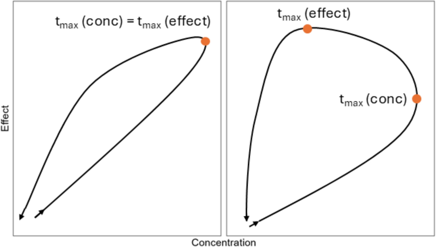
With hysteresis, effect on QTc increases more slowly than the concentration and remains after the drug concentration decreases. Hysteresis patterns may have very different shapes (Fig. 1). The directional pattern shows a counterclockwise relationship [11]. Identical concentrations have larger effects in the late phase compared to the early phase after drug administration.

Fig. 1

Two different shapes indicating hysteresis. Left: no difference between time of maximum concentration and time of maximum effect; right: substantial difference. Lines: concentration-effect in timely sequence (arrows indicate direction); orange bullets: times of maximum concentration and/or maximum effect; conc: concentration; tmax (conc/effect): time of maximum drug concentration/effect

Models such as the linear model assume a direct and immediate effect of the concentration on QTc interval duration and can, therefore, not be used if hysteresis is present because it violates the model assumptions. Of particular importance is the possibility that the time of maximum concentration may be substantially different from the time of maximum effect. Diagnosis of hysteresis can be based on population averages or individual ΔQTc versus concentration plots, as depicted in Fig. 1.

With circadian variation in QTc, ΔQTc based on a single baseline measurement may lead to false conclusions about hysteresis, ie, ΔQTc varying with the time of day [13]. Such limitations can be overcome with time-matched baseline data, i.e., 24-h QTc measurements at the same nominal times prior to treatment start. In such cases, ΔQTc is defined as the time-matched change from baseline, the difference between QTc after treatment start and QTc at baseline at the same time of day. Obviously, hysteresis can only be present in subjects on active treatment. Alternatively, presence of hysteresis can be assessed by comparing the goodness of fit for a direct-effect model to a model with effect compartment.

If hysteresis is present, it might be caused by an active metabolite that exerts an effect on QTc such that the time delay between parent concentration and effect change actually describes the metabolism from parent drug to metabolite with the effect originating from the metabolite. With metabolite concentration data, a metabolite-QT model with direct effect can be fitted and compared to a hysteresis model built on only parent concentration. Alternatively, a model where both compounds exert a direct effect on the QT interval can be fitted and the contributions of both compounds to the effect be assessed [2, 4]

In absence of such knowledge or data, hysteresis can be described by an effect-compartment model for the parent compound concentration. The effect compartment serves as the delay descriptor and the time delay is driven by the rate parameter that builds up the effect (Table 1).

The effect-compartment model is implemented as:

$$}/}\left( }} \right) \, = \, (/\tau_ )*\left( } - }} \right)$$

$$\Delta } = \, _ + }*}$$

with τ0 denoting the time with which the (virtual) concentration in the effect compartment, Ce, follows drug concentration in the central compartment, Cc [14, 15]; τ0 has time units whereby larger values of τ0 yield larger delays between concentration and effect change. The effect, ΔQTc, is described by an intercept, Θ0, and a slope for the relation between effect and concentration in the effect compartment, Ce. The statistical model for Θ0 and slope remains the same.

An example illustrates the role of the parameter τ0. In a 1-compartment linear PK model with ka = 0.7/h, kel = 0.05/h, V = 1L, and once-daily doses of 100 mg, the delay between change in concentration and change in effect, ΔQTc, increases with larger τ0. The time of maximum concentration after the first dose is 4.1 h. The times of maximum effect range from 5.5 h for τ0 = 1 to 23.8 h for τ0 = 25 over the first dosing interval to 29.1 h and 41.8 h (5.1 h and 17.8 h after dosing) for the second dosing interval (Fig. 2). The visualization of repeated doses shows that times of maximum effect after last dosing decrease with repeated doses (for all values of τ0).

Fig. 2

Hysteresis visualization: delayed ΔQTc (colors) and concentration (black) versus time for different values of τ0. The pharmacokinetic model was a 1-compartment model with ka = 0.7/h, kel = 0.05/h, V = 1L, and once-daily doses of 100 mg. Bullets indicate 4 different nominal times with identical concentrations, corresponding to the bullets in Fig. 3

The shapes of the hysteresis plots differ visibly, depending on the values of τ0. Furthermore, shapes and locations differ between first and subsequent doses (Fig. 3).

Fig. 3

Hysteresis plots for different values of τ0. Bullets indicate different nominal times with identical concentrations, corresponding to the bullets in Fig. 2

Model comparison

Common practice is to fit the linear regression model and inspect data and modeling results for violations of the model assumptions. Linearity is largely assessed visually, e.g, by inspecting a visualization of ΔQTc versus concentration or, post-hoc, residuals versus concentration supported by, e.g, a polynomial fit or a locally weighted scatterplot smoother [16, 17].

While a linear model frequently describes the concentration-QT data reasonably well, alternatives are generally not considered unless there is sufficient evidence that an assumption does not hold. On the opposite, pharmacometric analyses commonly compare model alternatives by visual assessments of predicted versus observed data and VPCs [9, 18] as well as by numerical measures of goodness of fit. Numerical assessments are based on likelihood comparisons. The likelihood expresses numerically the proximity of the model predictions to the observed data and generally increases with higher model complexity (number of parameters). To gauge if higher model complexity is warranted, the likelihood is counterbalanced by a penalty term for the number of parameters, leading to information criteria such as Akaike’s information criterion (AIC) [19], the BIC [20], and the BICc [10]. If the increase in likelihood is marginal compared to the higher model complexity, the simpler model is preferred, ie, the model with lower information criteria.

Decisions for model selection tend to be similar between AIC, BIC, and BICc. In the following, BICc is employed for model comparison because of its specificity for mixed-effects models with different penalty terms for fixed and random effects.

Dataset characteristics

The QT interval is known to exhibit diurnal variation, i.e., repeating patterns over the course of a day [21, 22]. Baseline-corrected QTc, i.e., ΔQTc, can be derived in several ways. Ideally, the analyses are based on time-matched ΔQTc with baseline data available as 24-h QTc profiles prior to drug administration. Change from baseline in QTc is derived by subtracting the time-matched baseline measurement from the QTc measurement after drug administration. This, on average, eliminates the circadian variation in ΔQTc.

If only a single baseline measurement is available, circadian variation can be modeled, e.g, as a cosine curve with parameters time shift and amplitude. Alternatively, a time component with time as a categorical covariate may be included into the model (as done in the white paper model), adjusting for each nominal time individually instead of employing a continuous curve. With circadian variation in ΔQTc, it can be expected that some corresponding nominal time parameters are different from 0. The placebo correction in ΔΔQTc removes the time component again.

In a study setup where placebo and active drug are administered to different subjects, e.g, in entry-into-man or parallel-group studies, baseline correction may be conducted based on the average placebo response per nominal time.

Overall, the definition of the change from baseline (single baseline value or time-matched change from baseline on the individual level or on the aggregate level using average placebo values) as well as the centered baseline affects the data set preparation from the raw data but not the modeling process as such.

Implementation

Mixed-effects regression models (linear and nonlinear) were employed for all analyses. Model parameters were estimated using the stochastic approximation expectation–maximization (SAEM) algorithm. All models were implemented in Monolix 2024R1 [23]. Calculations of CIs were performed using Simulx 2024R1 [24]. Monolix and Simulx were used through the lixoftConnectors package [25], which provides an application programming interface (API) from R for the MonolixSuite. R version 4.4.2 [26] was used, and an R quarto script [27] (quarto version 1.5.57) served as a wrapper to create the output as Word files. The Monolix models can be fitted from the GUI version, too, by opening the corresponding mlxtran files.

The R functions allowing to (1) format an input dataset for analysis, (2) generate Monolix projects to run a conc-QTC analysis using the standard linear model as well as alternative non-linear models and (3) generate a report as Word document can be downloaded from https://monolixsuite.slp-software.com/r-functions/?contextKey=package-conc-qtc. Example of usage and results for the 4 compounds in Johannesen et al. [28] are also provided on the webpage.