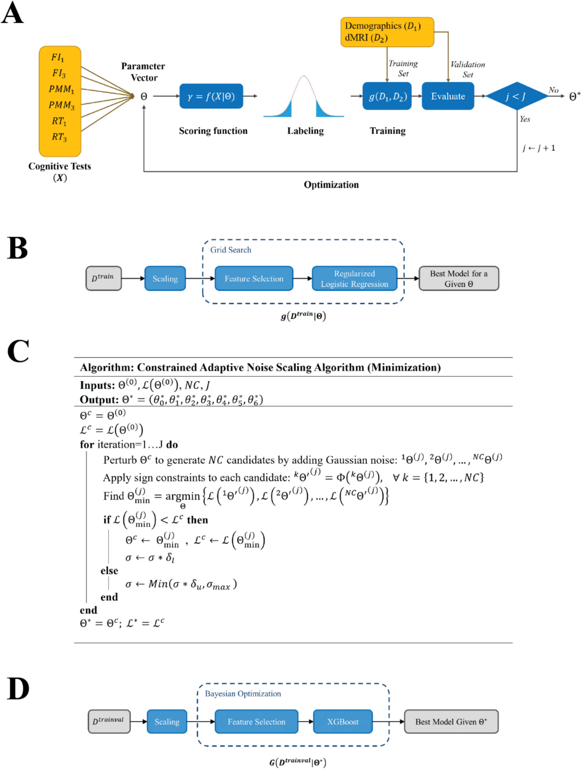
In this section, we begin by analyzing the numerical results and comparing the performance of the proposed algorithm with that of the baseline models. Subsequently, we evaluate feature significance using SHapley Additive exPlanations (SHAP) values. SHAP values offer a comprehensive method for interpreting the contribution of individual features to the classification outcomes, thereby enabling us to identify which variables have the most significant impact on the algorithm’s predictions. Following this, we outline the validation steps undertaken to ensure the effectiveness of the scoring function. We then conduct a post-hoc analysis to explore the optimal scores generated by the proposed algorithm. This analysis includes a detailed comparison between Positive-Agers and Cognitive Decliners with respect to dMRI features and demographic data. Finally, we address the question: “Is it possible to predict future trajectories using only the baseline visit data?”.

Numeric results for cognitive classification

Here, we present a comparative analysis of the proposed algorithm against baseline models, with the results summarized for different quantile thresholds in Table 1. We categorized our findings into the following subsections:

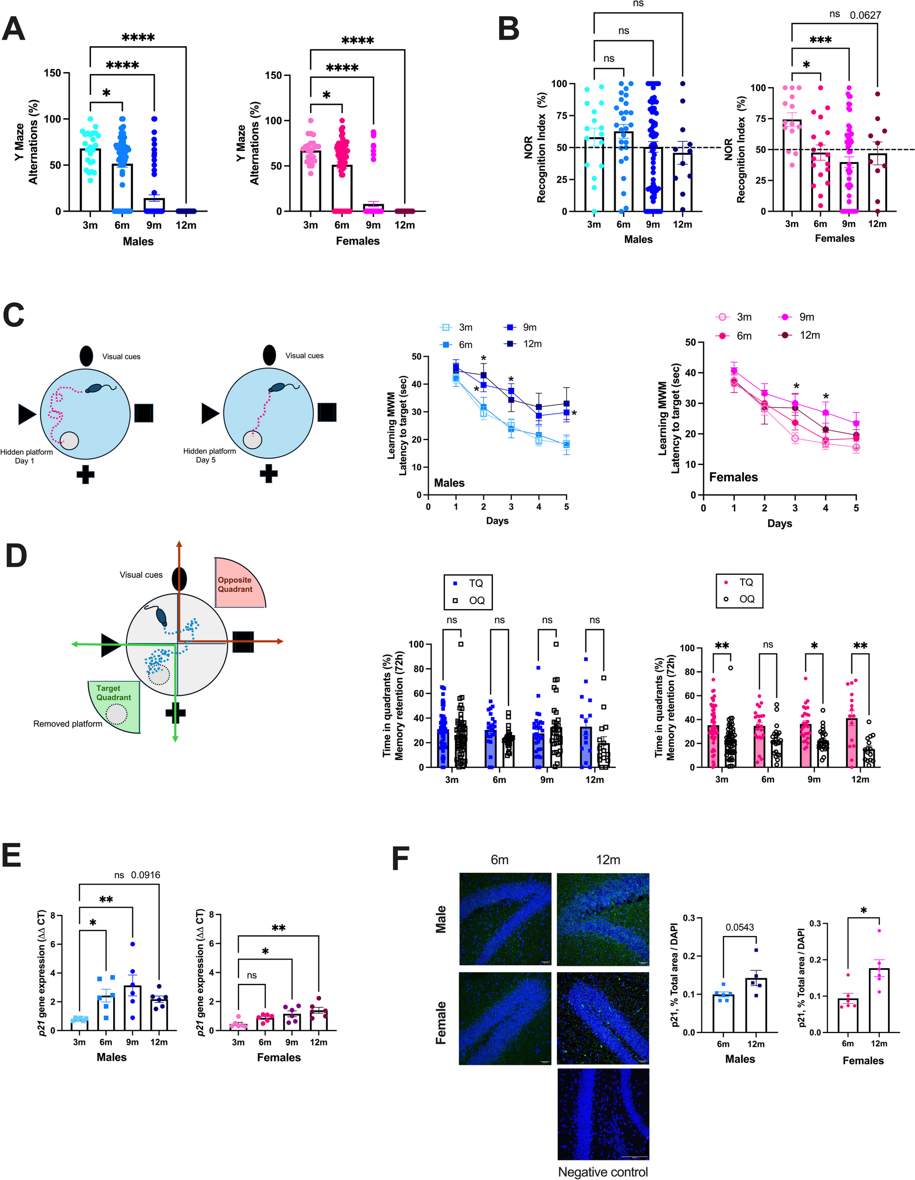
Table 1 Classification results for predicting cognitive classes Optimal quantile threshold

Using a quantile threshold of \(q\) = 0.15 yielded the highest AUC value, reaching 83% (see Fig. 2A for the ROC curve comparison). This suggests that increasing the threshold further introduces noise into the labeling procedure by including individuals who may not belong to the “Cognitive Decliner” or “Positive-Ager” class and may be Normal-Agers. Thus, \(q\) = 0.15 appears to be the optimal balance, minimizing the inclusion of noise and enhancing the classification accuracy. In this setting, we achieved an accuracy of 72%, a precision of 74%, a recall value of 71%, a specificity of 74%, and an F1-score of 72%.

Fig. 2

Evaluating the performance of the algorithm and feature contribution. A ROC curves for the algorithm and baseline models for \(q\) = 0.15. B Feature importance for the top 30 features using the mean of absolute SHAP values. C SHAP values for the top 30 features. D Total aggregated importance of dMRI feature sets

Performance consistency

The proposed algorithm consistently outperformed the baseline models in terms of AUC, regardless of the chosen quantile threshold. Additionally, the proposed algorithm demonstrated superior performance across other metrics within each quantile category. It is important to note that the baseline models share foundational similarities with the proposed algorithm, which means they may not serve as entirely independent benchmarks. Nevertheless, in the absence of relevant frameworks in the literature, these designed baselines are valuable for assessing the methodology’s effectiveness, particularly in terms of feature inclusion and the optimization loop.

Feature inclusion

When comparing the full algorithm with the “dMRI Only” and “Demographics Only” baseline models, it is evident that the combination of dMRI and demographic data is essential for achieving maximum performance. While utilizing only dMRI features and ignoring demographic characteristics significantly decreased the performance metrics across all threshold categories, relying solely on demographic features did not result in as severe an accuracy loss as the “dMRI Only” model. However, after adding the dMRI features to the “Demographics Only” model, the AUC improved by 7% and specificity also increased by 6%. Please refer to the Supplementary Text: Sect. 3A for explanations about why the exclusion of the dMRI subset was conceptually and methodologically not tenable.

Optimization

Comparing the results between the “PCA” model and the full algorithm shows that using the optimal parameter vector enhanced overall performance.

Contribution of features in cognitive classification

We used SHAP values to quantify the contribution of features for the final prediction. Figure 2B illustrates the average of absolute SHAP values for the top 30 features. The higher the mean absolute SHAP value, the larger the magnitude of the average impact will be for a particular feature. Among the demographic variables, education, age, waist circumference, and sex were the most influential features. In the dMRI dataset, the top six features were “mean MO in fornix cres + stria terminalis,” “mean L1 in medial lemniscus,” “mean OD in cerebral peduncle,” “mean L3 in cerebral peduncle,” “mean L1 in tapetum,” and “mean L1 in superior cerebellar peduncle.”

Plotting SHAP values can also be insightful because it helps us understand the direction of the effect for each variable, as well as the spread of the effect. Figure 2C shows the SHAP values for the top 30 features. There were several interesting findings: (I) Individuals with a low level of education were less likely to be “Positive-Agers.” This negative effect became stronger as the level of education decreased. (II) Aligned with our expectations, general cognitive performance decreased as people age. This can be concluded since older individuals have negative SHAP values showing a decrease in the predicted probability of being a Positive-Ager. (III) Men were more likely to be Positive-Agers. (IV) As waist circumference increases, the predicted probability of being in the “Positive-Ager” class increases in general (see the “Discussion” section for a more comprehensive analysis). (V) Individuals with higher values of “mean MO in fornix cres + stria terminalis” and “mean L1 in medial lemniscus” are more likely to be Positive-Agers, while individuals with higher values of “mean OD in cerebral peduncle” are less likely to be Positive-Agers (see detailed analysis in the “Analysis of dMRI attributes” section).

We plotted the aggregated feature importance, which helped us identify the effect of various dMRI attributes. For this purpose, we summed up the mean absolute SHAP values corresponding to any of the dMRI attributes (see Fig. 2D). We also plotted the aggregated SHAP values for various regions of interest in the brain, which is shown in Supplementary Fig. S2.

Cognitive scoring function

Despite the intricacies of the internal workings of the algorithm, the final output is a straightforward and interpretable mathematical equation. This equation can be utilized to quantify an individual’s cognitive score based on longitudinal cognitive assessments. This is expressed as

$$\gamma =f\left(X \right| ^)=\sigma \left(^X\right)=\frac^^X }}$$

(18)

where \(^X\) is

$$^X=-0.622+1.764\left(\frac_-6.86}\right)+ 2.198\left(\frac_-6.79}\right)-0.349\left(\frac_-1.40}\right)-1.371\left(\frac_-1.41}\right)-0.633\left(\frac_-6.32}\right)-1.191\left(\frac_-6.40}\right)$$

(19)

Here, \(F_, F_, \dots , R_\) are the original exam values, which are standardized in parentheses with the corresponding means and standard deviations found during the training process. The labels are then assigned based on the lower and upper bounds obtained by the algorithm:

$$y=\left\`\!\ \!`Cognitive\;Decliner\!",if\gamma\leq0.004\\`\!\ \!`Positive-Ager\!",if\gamma\geq0.986\\`\!\ \!`Normal-Ager\!", otherwise\end\right.$$

(20)

There are several interesting facts about the yielded cognitive scoring function. First, by comparing the coefficient magnitudes at \(_\) and \(_\) for each cognition test, it can be observed that the algorithm emphasized more on the test results collected on the third visit (\(_\)). This makes sense because the dMRI attributes are also collected at the third visit. In addition, time point \(_\) provides the most recent assessment of participants’ cognitive performance. The algorithm already made proper adjustments accordingly. Second, the lower and upper bounds proposed by the algorithm are very close to the two ends of the cognitive scores’ interval (i.e., [0, 1]). This highlights that the algorithm effectively determines the scores, ensuring that the extreme groups are positioned at the very ends of the interval. It assigns labels only when there is clear evidence for an individual to belong to a specific cognitive group, indicating algorithm robustness. Figure 3A shows the histogram of cognitive scores calculated for the participants in this study. It can be observed that Positive-Agers and Cognitive Decliners are at the two ends of the score’s interval, depicting a perfect separation. Third, according to weight magnitudes, fluid intelligence is the most influential cognitive test, as the weight associated with this exam is the largest in absolute value. The RT and PMM tests were the second and third most influential tests. Fourth, the baseline score for someone performing the same as the average population on all tests is \(\sigma\)(\(-0.622)\approx 0.35\). This value seems reasonable, as we generally anticipate a decline in cognitive performance over time in the population. Therefore, having the baseline score closer to the “Cognitive Decliner” group makes sense.

Fig. 3

Comparison of cognitive exams between different cognitive classes. A Histogram of optimal cognitive scores (\(\gamma\)). Positive-Agers and Cognitive Decliners are at the two ends of the score range. B Boxplot of the average cognitive exams of \(_\) and \(_\) for Positive-Agers and Cognitive Decliners. C Estimated kernel density plots of cognitive tests for Positive-Agers and Cognitive Decliners at each visit, separately. D Boxplot of cognitive tests for an independent sample of 1482 participants who were not included in any part of the study (FI, fluid intelligence; PMM, pairs matching memory; RT, reaction time)

The proposed cognitive scoring system offers several benefits. First, although we excluded the middle group (i.e., “Normal-Agers”) and focused on distinguishing between two extreme cognitive classes, the framework provides a continuous scoring mechanism that captures the entire range of cognitive performance. Specifically, if the computed cognitive score falls between 0.004 and 0.986, the individual belongs to the “Normal-Aging” group. Second, the current configuration maps cognition test results to a restricted interval between 0 and 1. This makes the score an interpretable metric that is easy to compare across individuals in a population. Third, the score’s range is fixed and independent of the population or cognitive exam values observed. This provides researchers with a mechanism to make comparisons across different populations concerning the distribution of cognitive performances and their characteristics. This, however, requires validation on independent samples first.

Sensitivity analyses: validation of scoring system

Here, we examined whether the proposed cognitive scoring system produces reasonable scores or not. For this purpose, we conducted two sets of analyses. First, we compared the cognitive tests for individuals labeled as “Positive-Ager” against those identified as “Cognitive Decliners” by the algorithm. This assessment checks whether there is a clear separation between two cognitive classes in terms of cognitive performance or not, regardless of any additional input features. Table 2 summarizes the cognitive test’s mean and standard deviation at time points \(_\) and \(_\) for the two cognitive groups. An independent t-test was conducted to examine the difference in the mean levels. The P-values for all tests were significant, and the effect size calculated depicted a large effect size. This clearly indicates that the two classes significantly differ with respect to cognitive performance and verifies the algorithm’s effectiveness in creating such a separation. One interesting observation is that, in moving from \(_\) to \(_\), the absolute difference in the mean levels of the two classes and the corresponding effect size increases. This implies that the cognitive gap between the two classes increases as the population ages. The distribution of mean cognitive exams and individual tests between the two cognitive classes are shown in Fig. 3B, C, respectively. We noticed that FI tests were most effective in creating such a separation. This is aligned with our previous finding in the “Cognitive scoring function” section, where FI tests had the largest weight magnitudes in the optimized parameter vector found by the algorithm.

Table 2 Descriptive statistics of cognitive tests for “Positive-Agers” vs. “Cognitive Decliners”

For the second set of validation experiments, we utilized an independent sample comprising cognitive test results from 1482 participants who were not included in any part of the study due to the unavailability of dMRI data. To enhance the robustness of the analysis, we incorporated additional cognitive exams such as the symbol digit substitution test, the maximum digits remembered test (i.e., numeric memory test), and the trail-making tests A and B (see Supplementary Text: Sect. 3B for further details on the definition of new exams). Using the same scoring function, we assigned cognitive labels to each participant. Figure 3D displays the boxplots for each cognitive test corresponding to this independent sample. As before, a clear distinction was observed between the mean levels for each cognitive exam.

In conclusion, both sets of analysis corroborate the algorithm’s effectiveness in distinguishing between the cognitive classes of “Cognitive Decliner” and “Positive-Ager.”

Analysis of demographic characteristics

The summary statistics of demographic attributes for the two cognitive classes can provide valuable insights and is summarized in Table 3. We plotted the distribution of the most important demographic features, including education, age, waist circumference, and sex in Supplementary Fig. S3.

Table 3 Descriptive statistics for demographic features

For a detailed analysis of sex dimorphism in demographic features, please refer to Supplementary Table S4.

Analysis of dMRI attributes

dMRI is one of the primary feature sets employed by the classifier to differentiate between the “Cognitive Decliner” and “Positive-Ager” classes. To elucidate the differences in dMRI attributes across these groups, we compared the values of the top dMRI features. Figure 4A presents violin plots for the top six regions of DTI data, highlighting the disparities between the two groups. An independent t-test conducted on participants in the test set (\(n\) = 270) revealed significant differences at the 5% significance level between the mean levels of these cognitive classes for each dMRI attribute, except for “mean L1 in medial lemniscus,” where the mean values were nearly identical (difference of 3.6e-6); hence, the test was not able to detect mean differences. Boxplots for the remaining regions are provided in Supplementary Fig. S4.

Fig. 4

Analysis of the top six dMRI features using participants in the test set. A Violin plot of top six dMRI attributes for Positive-Agers and Cognitive Decliners. An independent t-test was conducted, and the P-values are reported on top of each violin plot (***P < 0.001; **P < 0.01; *P < 0.05; ns, non-significant). Values in parentheses are the absolute values of Hedge’s g effect. B Scatter plot of top six dMRI attributes against their SHAP values. The rank of a feature represents its relative position among all existing variables based on its importance

Having examined the differences between the two optimal classes identified by the algorithm, it is insightful to explore the relationship between dMRI attributes and the likelihood of positive-aging as the next step. Figure 4B presents scatter plots of SHAP values against the values of the top dMRI features. The analysis uncovered that mean MO in the fornix + stria terminalis, mean L1 in the medial lemniscus, and mean L1 in the superior cerebellar peduncle exhibit a positive correlation with the likelihood of positive aging. Conversely, the other three attributes, including mean OD and mean L3 in the cerebral peduncle and mean L1 in the tapetum, show a negative correlation. Below, we explore the details of the direction and magnitude of the impact for each of these dMRI attributes:

Mean MO in fornix + stria terminalis on FA skeleton

We observed that mean MO values in the fornix and stria terminalis tracts greater than 0.58 were associated with approximately a 2% increased likelihood of being a Positive-Ager. Conversely, values smaller than 0.45 decreased this likelihood by up to 7% in some participants.

Mean L1 in medial lemniscus on FA skeleton

There is a positive linear relationship for values larger than 0.00135, with an up to 4% increase in the likelihood of positive aging. Values smaller than this threshold are associated with a decrease in the likelihood of positive aging, with a mean impact of around 1%.

Mean OD in cerebral peduncle on FA skeleton

Values larger than 0.104 were associated with a decrease in the positive aging likelihood, while values smaller than this threshold increased this likelihood. This impact can be up to 2.5% in both directions.

Mean L3 in cerebral peduncle on FA skeleton

Values less than 0.0029 in the crus cerebri did not have a significant impact (maximum impact of 1%). However, values higher than this threshold were associated with a decrease in the likelihood of positive aging by up to 5%.

Mean L1 in tapetum on FA skeleton

Axial diffusivity values less than 0.0017 were associated with an increased positive aging likelihood, while values higher than this threshold had a negative impact of up to 2%.

Mean L1 in superior cerebellar peduncle on FA skeleton

Values higher than 0.00157 are positively correlated with the likelihood of positive aging, whereas values less than this cutoff were associated with a decrease in this likelihood by up to 3%.

The scatter plot of the impact for the remaining dMRI attributes is shown in Supplementary Fig. S5.

Longitudinal analysis of cognitive trajectories

Although the proposed methodology has provided a powerful yet straightforward mechanism to quantify individuals’ cognitive performance, equipping the algorithm with tools to study cognitive trajectories and rates of change may offer additional insights into how cognitive capabilities evolve over time.

Considering the scoring system proposed, we can decompose it into three independent components:

Here, \(_^\) and \(_^\) are called adjusted scores at \(_\) and \(_\), respectively. The term “adjusted” refers to the fact that scores are computed based on the optimal weights obtained from the algorithm’s output:

$$_^=_^ F_^+_^ PM_^+_^R_^$$

(22)

$$_^=_^ F_^+_^ PM_^+_^R_^$$

(23)

We plotted the cognitive trajectories using \(}_^\) and \(}_^\) in Fig. 5A. The figure illustrates a clear separation between different cognitive groups in terms of both the trajectory’s starting points and its slope: Positive-Agers are located in the positive zone and generally exhibit more positive slopes, indicating an upward trend in their cognitive trajectories as expected. Conversely, Cognitive Decliners are situated in the negative zone and demonstrate a downward trend. Individuals classified as Normal-Agers fall in the middle, with slopes close to zero, scattered around the zero mark.

Fig. 5

Analysis of cognitive trajectory and the corresponding slopes. A Cognitive trajectories plotted based on \(_^\) and \(_^\). The color of each line represents the corresponding cognitive class to which an individual is assigned (red: Cognitive Decliner; orange: Normal-Ager, and green: Positive-Ager). B Scatterplot of \(_^\) and \(_^\) with respect to the cognitive score, \(\gamma\), calculated. C Scatter plot of \(_^\) and \(_^\) with respect to adjusted trajectory slopes, \(_\). D Boxplot of adjusted trajectory slopes at different levels of baseline age. E Scatter plot and regressed line of the average adjusted trajectory slope against baseline age. F Constructed average cognitive trajectory curve for different cognitive groups. Dashed lines are straight lines that aim to better visualize the main trajectory path. G Scatter plot of \(_^\) and \(_^\) with respect to the cognitive classes. H The heatmap of the expected slope, given the initial adjusted score and age (\(_^\), adjusted score at \(_\); \(_^\), adjusted score at \(_\); \(_\), adjusted trajectory slope)

After this reformulation, we can rewrite the definition of Cognitive Decliners as below:

$$\frac^_^+_^+_^\right)}}\le lb$$

(24)

which can be simplified as

$$_^\le -_^-_^+\text\left(\frac\right)$$

(25)

After substituting \(_^\) and \(lb\) with the optimal values shown in (19) and (20), that is \(_^=-0.622, lb=0.004\), we have the optimal inequality corresponding to the definition of Cognitive Decliners:

$$_^\le -4.9-_^\;OR\;_^+_^\le -4.9$$

(26)

This implies that if the sum of adjusted scores from the two visits is − 4.9 or lower, the participant is classified as a Cognitive Decliner. Equivalently, for a given initial visit with an adjusted score \(_^=s\), the highest possible score in the next visit that will still categorize the individual as a Cognitive Decliner is \(-4.9-s\).

Applying the same procedure to the “positive-aging” definition, we have

$$_^\ge -_^-_^+\text\left(\frac\right)$$

(27)

Substituting \(ub=0.986\) and \(_^=-0.622\) will result in the following inequality:

$$_^\ge 4.9-_^\;OR\;_^+_^\ge 4.9$$

(28)

This means that if the sum of adjusted scores from the two visits is 4.9 or higher, the participant is classified as a Positive-Ager. Equivalently, for a given initial visit with an adjusted score \(_^=s\), the lowest possible score in the next visit that will place the individual into the Positive-Ager class is \(4.9-s\). Supplementary Fig. S6 shows the corresponding line equations.

Another advantage of the reformulation in Eq. (21) is that we are now able to analyze the rate of change in cognitive performance for a given participant using Eq. (29).

This new variable, \(_\), is termed the adjusted trajectory slope. To understand the rationale behind using the adjusted trajectory slope instead of other forms, refer to Supplementary Fig. S7. This figure compares various approaches to computing the rate of change and demonstrates that optimal weights in the adjusted scores provide the best separation between cognitive classes. The relation between \(_^\) and \(_^\) with cognitive score (\(\gamma\)) and trajectory slope (\(_\)) is shown in Fig. 5B, C, respectively. For a deeper analysis of the relationship between the computed cognitive scores and adjusted trajectory slope, refer to Supplementary Fig. S8.

Studying the trajectory slope in different age groups may provide additional insights. For this purpose, we plotted the boxplot of the adjusted trajectory slope for cognitive groups at different levels of baseline age in Fig. 5D. As the plot suggests, there is a significant difference in the mean level of adjusted cognitive slopes across the three cognitive groups. Additionally, we observed a consistent pattern: on average, regardless of baseline age, individuals in the positive-aging group have a positive slope, individuals in the Cognitive Decliner group have a negative slope, and those in the Normal-Aging group have a slope value close to zero. This observation leads to the question, “How does the slope change as people age, then?”. Figure 5E addresses this by plotting the average adjusted trajectory slope (\(}_\)) against baseline age. We used robust linear regression to capture the linear trend in the data while ignoring outlier data points. Several interesting observations emerged: First, on average, trajectory slopes decreased as people age. Also, this figure suggests that individuals with improving trajectories experience less improvement over time, while those with declining cognitive performance experience greater cognitive decline. Second, comparing the age coefficient in the regressed lines, we noticed that the magnitude of changes in Cognitive Decliners was about 2.5 times that of Positive-Agers, indicating that the change in the rate of cognitive decline was significantly steeper than that of cognitive improvement as people age.

Constructing the average cognitive trajectory curve

In Fig. 5E, we analyzed the average trajectory slope given a baseline age. The points on that plot can be viewed as the derivative of a primary average cognitive trajectory curve at different age levels (i.e., years of age). Our aim here is to construct the cognitive trajectory curve using the observed derivative values for each cognitive class. Suppose Eq. (30) represents the line equation for the trajectory slope:

By integrating this equation, we can obtain the average cognitive trajectory curve, denoted as \(\mathcal\):

$$\mathcal=\int (mt+b)dt=\frac^}+bt+u$$

(31)

where \(u\) is a constant and was replaced with the average \(_^\) at the initial baseline age for this subset of UK Biobank data (55 years). Figure 5F shows the estimated average cognitive trajectory for each group based on the observed data. The dashed lines are plotted alongside the curves to compare them with the corresponding straight lines, providing a clearer visualization of the changes in cognitive performance over time. This figure suggests that as people age, the gap in cognitive capability between Positive-Agers and Cognitive Decliners increases. This observation aligns with our previous findings in the “Sensitivity analyses: validation of scoring system” section, where we compared the absolute difference in mean cognitive exam levels at \(_\) versus \(_\) (see Table 2). The resulting mathematical equations for each cognitive class are presented in Supplementary Text: Sect. 3C.

Predict cognitive trajectory on the first visit

This study utilizes longitudinal data. However, deriving insights solely from the baseline visit to forecast future trajectories could be beneficial in identifying individuals’ cognitive categories in advance. To this end, we initially plotted \(}_^\) and \(}_^\) in relation to different cognitive classes, as illustrated in Fig. 5G. Several significant observations emerged. First, individuals with a positive initial adjusted score were highly unlikely to be classified as “Cognitive Decliners,” while those with a negative \(}_^\) are rarely “Positive-Agers.” Second, all individuals with \(}_^\ge 5\) were identified as “Positive-Agers” regardless of their subsequent assessments, and those with \(}_^\le -5\) were predominantly “Cognitive Decliners,” with only one exception. This pattern holds true for the interval between visits in this study. The subsequent boundaries, \(_^=2.16\) and \(_^=-2.10\), shown in Fig. 5G, were determined by minimizing the Gini index and representing the optimal split points for identifying cognitive groups. Individuals with initial adjusted scores higher than 2.16 are more likely to be “Positive-Agers,” while those with scores lower than − 2.10 are more likely to be “Cognitive Decliners.” Participants with scores between these thresholds are mostly “Normal-Agers.”

Next, we investigated the possibility of estimating the trajectory slope using the baseline age and initial adjusted score, \(_^\) (see Fig. 5H). The plot presents a heatmap of the expected slope for a given initial adjusted score (\(s\)) and baseline age (\(t\)). The expected slope at each point is computed based on the mean slope observed for participants aged \(t\), whose \(_^\) was within 0.25 of the value \(s\) (i.e., within the interval \([s-0.25, s+0.25]\)). Furthermore, we imposed a requirement of having at least ten participants in that range to estimate the mean slope. Several notable observations can be drawn from this figure. First, individuals with negative scores in their 5th decade of life (i.e., 50s) are more likely to show improvement over time compared to those with similar scores in their late 60s. Second, a general decline is observed in the late 60s, irrespective of the initial score, when compared to individuals in their 50s. Third, participants with very high scores (\(_^\) values close to 4) tend to experience a general decline in their cognitive scores over time. This may suggest that improvement beyond such high scores is improbable within this age range, suggesting that individuals either maintain the same level of cognitive performance or experience a decline over time.

As the final step, we utilized all available baseline data, including demographic information and exam results, to predict the cognitive classes: “Positive-Ager,” “Cognitive Decliner,” and “Normal-Ager.” A decision tree model was trained on the same data used in developing the algorithm, and its accuracy was evaluated on the independent sample described in the “Sensitivity analyses: validation of scoring system” section, which has not been utilized in any part of the study. The model achieved an accuracy of 79% using only the information from the first visit. The decision tree diagram and the corresponding confusion matrix are shown in Supplementary Fig. S9. The confusion matrix indicates that the model did not misclassify “Cognitive Decliners” as “Positive-Agers” and vice versa.