Number of neuronal activations in CA1 hippocampal neurons is stable over time and is affected by acute stress

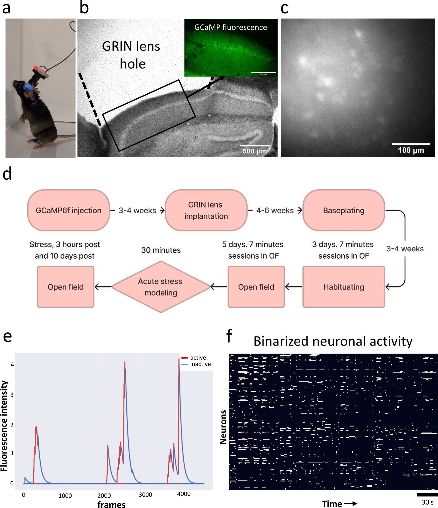
To assess the stability properties of the hippocampal neuronal ensembles under both normal conditions and after external stimulus, a miniature fluorescent microscopy method was performed on the 8 month old C57BL/6J mice line (Fig. 1a). To record activity of excitatory hippocampal neurons genetically encoded calcium-sensitive fluorescent indicator GCaMP6f was used (Fig. 1b, c). Miniscope method allows us to record hundreds of neurons over days with stable field of view (Fig. S1) [34]. The CA1 hippocampal neurons state was recorded in freely moving sessions once a day for five consecutive days, serving as a baseline reference. In the current manuscript, we used terms “neuronal circuits” or “neuronal ensembles” for the identification of the group of CA1 neuronal cells that were imaged with the miniscope. To induce an external shift of hippocampal activity, the mice underwent a 30-min acute stress modeling. Then the neuronal circuits activity was recorded immediately after the stress test (referred to as “stress” in all graphs), as well as 3 h (“3 h”) and 10 days (“10 days”). The overall timeline is presented in Fig. 1d. All the data were processed using the “spike” method (Fig. 1e), where only the rapid phase of the calcium indicator signal growth was considered unless otherwise specified. For analysis we have transformed all the neuronal activity into binarized activity (Fig. 1f) [32].

Fig. 1

Experimental pipeline schematic presentation. a Freely behaving mouse with an attached miniscope v3. b Fixed sagittal brain slice with hole above the hippocampus after surgery, 4× magnification (in the right corner fluorescent image of the GCaMP6f fluorescence, 10× magnification). By dotted line GRIN lens boarders are drawn. c CA1 hippocampal neurons activity recorded by the miniscope. Illustration represents sum of 1000 frames from a single recording. d Timescale for neuronal activity visualization by miniscope in the Open-field behavioral test with acute stress modeling as a great external stimulus. e Extracted single neuron activity as active and inactive state using spike method with values “warm” of 50 and “cold” of 0 in “NeuroActivityToolkit”. f Recorded neuronal ensembles activity representation in a binarized form for a single recording (mouse 1, baseline day 1, 182 neurons). White lines indicate single neuron activation

To validate this statement and confirm whether neuronal activity returns to a stable original point after recovery, we analyzed the mean values of individual neuronal activations. In this case, the overall activity of the neuronal circuits is characterized by the mean level of all neuron’s activity in this network. It can be clearly observed that right after stress and at the 3-h post time point the hippocampal ensembles are in an excited state since the number of activations per minute is elevated (1.27 ± 0.05, n = 15 (baseline) vs 2.48 ± 0.48, n = 3 (stress), p = 0.0002; 1.27 ± 0.05, n = 15 (baseline) and 2.32 ± 0.33, n = 3 (3 h), p = 0.0009, F(3,20) = 14.29, One-way ANOVA with following Tukey post-hoc test). Moreover, by day 10, the activity of the hippocampal neurons returned to its initial value with no significant differences observed with baseline values (1.27 ± 0.05 (baseline) and 1.36 ± 0.13 (10 days), p = 0.9690, F(3,20) = 14.29, One-way ANOVA with following Tukey post-hoc test) (Fig. 2d). For a more detailed visualization, binarized activity of the neurons in all states can be found in Fig. S2(a). Considering the natural variability among individual mice, we have also performed normalized per-mouse analysis of activations per minute (Fig. S3), where the similar changes are stated. Further, to examine neuronal activations at the single-neuron level, we tracked the activity of the neurons shared between the baseline level (day 5) and across stress, 3 h and 10 days states. We have determined significantly increased activity of the same tracked neurons between sessions, consistent with the overall circuits activation as shown above. A great elevation of neuronal activations was observed during the stress state (1.34 ± 0.11, n = 73 neurons (baseline) vs 2.51 ± 0.14, n = 73 neurons (stress), p < 0.0001) and at 3 h state (1.34 ± 0.11, n = 73 neurons (baseline) vs 2.33 ± 0.11, n = 64 neurons (3 h), p < 0.0001). Moreover, no significant changes were observed 10 days post stress modeling (1.34 ± 0.11, n = 73 neurons (baseline) vs 1.37 ± 0.09, n = 64 neurons (10 days), p > 0.9999) (Fig. 2g). While addressing normalized individual response from the shared neurons between sessions, the same tendency was observed (Fig. S3(b)). To validate how acute stress modeling influenced hippocampal neurons, we have analyzed neuronal activations changes in all states. Firstly, we have identified threshold levels for “stress activated” and “stress inhibited” neurons (see Materials and Methods section). Then, activity of the same neurons for stress, 3 h and 10 days states was normalized on the baseline level. We have found that 62.87% of the shared neurons were stress activated, 11.42% stress inhibited and 25.71% did not respond to stress. At the same time, at 3 h mark stress activated neurons relative amount was 49.25, 8.96% were stress inhibited and 41.79% of neurons were stress non-responsive (Fig. 2f). 10 days after great external stimuli, we have identified, that only 28.81% of neurons were stress activated, while activity of 23.73% neurons was inhibited and 47.46% did not respond to stress. Representative calcium traces of the same stress activated, stress inhibited and stress-non responsive neurons across sessions can be found in Fig. 2g.

Fig. 2

Shift in the activity properties at the single neuronal level as well as in the entire neuronal ensembles after acute stress modeling. a–c Calcium events number per minute for individual mouse for single-cell activity comparison. d Mean value of calcium events as total neuronal circuits characteristic for all states (baseline (n = 15) vs stress (n = 3), p = 0.0002; baseline (n = 15) vs 3 h (n = 3), p = 0.0009; baseline (n = 15) vs 10 days (n = 3), p = 0.9690; stress (n = 3) vs 3 h (n = 3), p = 0.9467; stress (n = 3) vs 10 days (n = 3), p = 0.0066; 3 h (n = 3) vs 10 days (n = 3), p = 0.0212; Ordinary One-way ANOVA with Tukey test for multiple comparison, F(3,20) = 14.29). e Individual response from the shared neurons between sessions for all states. All comparisons are significantly different with p < 0.0001, except: stress (n = 73 neurons) vs 3 h (n = 64 neurons), p > 0.9999 and baseline (73 neurons) vs 10 days (64 neurons), p > 0.9999. f Percentage of neurons that responded to stress or not for stress, 3 h and 10 days states. (g) Left: representative calcium traces of the same stress activated neuron on day 5 (baseline), stress, 3 h and 10 days states. Middle: representative calcium traces of the same stress inhibited neuron on day 5 (baseline), stress, 3 h and 10 days states Right: representative calcium traces of the same stress non-responsive neuron on day 5 (baseline), stress, 3 h and 10 days states. Scale bars corresponds to 25 s. Kruskal–Wallis test with Dunn’s test for multiple comparisons was used for comparisons in a–e, ns: no significant difference, #: p < 0.05; ##: p < 0.01; ###: p < 0.001; ####: p < 0.0001. Ordinary one-way ANOVA following Tukey post-hoc test was implemented for comparison in d, *: p < 0.05; **: p < 0.01; ***: p < 0.001; ****: p < 0.0001. All the data presented as mean ± SEM

In conclusion, the averaged neuronal activity in the recorded hippocampal area can be stated as a stable value over days that reverts to its “home” state after reaction to a crucial external perturbation.

External stimulus induced by acute stress lead to severe changes in the hippocampal neuronal ensembles activity properties

To investigate dynamic shifts in the hippocampal neuronal network activity, we analyzed metrics related to neuronal activation characteristics. Our first focus was on comparing the distribution of neurons with the given number of activations to observe how strong was the total response of the circuits to the applied stimulus (referred to as the “burst rate”). We compare the distributions for baseline, “stress”, “3 h” and “10 days” which are presented in Fig. 3a–c. These comparisons indicated a noticeable increase in the number of neurons with a larger number of the calcium activations per minute, expressed in the difference in most data points under stressed conditions (Fig. 3a, b). Peak values for the baseline level ranged from 0.66 to 1.00 activation per minute, whereas for stressed conditions they reached 3.00–3.33 for the “stress” state (in comparison with baseline value: n = 15 for baseline and n = 3 for stress, p = 0.0206, Mann–Whitney test) and 2.66–3.00 (in comparison with baseline value: n = 15 for baseline and n = 3 for the “3 h”, p = 0.0029, Mann–Whitney test) for 3-h post stress time-point. At the same time, the distributions for baseline and 10 days post acute stress modeling were similar (Fig. 3c).

Fig. 3

Hippocampal neuronal ensembles activation properties in normal and perturbed conditions. Distributions of neurons percent with given number of activation in normal condition and a right after stress (baseline (n = 15) vs stress (n = 3): 0.66–1.00: p = 0.0403; 1.00–1.33: p = 0.0059; 1.33–1.66: p = 0.0029; 3.00–3.33: p = 0.0206; 3.33–3.66: p = 0.0029; 3.66–4.00: p = 0.0250; 4.33–4.66: p = 0.0235; 4.66–5.00: p = 0.0029; 5.00–5.33: p = 0.0103; 5.33–5.66: p = 0.0029; 5.66–6.00: p = 0.0015, Mann–Whitney test for all). b 3 h post acute stress (baseline (n = 15) vs 3 h (n = 3): 2.33–2.66: p = 0.0029; 2.66–3.00: p = 0.0029; 3.00–3.33: p = 0.0029; 3.33–3.66: p = 0.0029; 3.66–4.00: p = 0.0029; 4.00–4.33: p = 0.0015; 4.33–4.66: p = 0.0235; 4.66–5.00: p = 0.0029; 5.00–5.33: p = 0.0103; 5.33–5.66: p = 0.0059, Mann–Whitney test for all). c 10 days post acute stress (baseline (n = 15) vs 10 days (n = 3): 0.33–0.66: p = 0.0208; others are non-significant, Mann–Whitney test for all). Distributions of network spike rate metric in normal condition and d right after stress (baseline (n = 15) vs stress (n = 3): 0.0–2.5: p = 0.0018; 2.5–5.0: p = 0.0018; 10.0–12.5: p = 0.0044; 12.5–15.0: p = 0.0026; 15.0–17.5: p = 0.0044; 17.5–20.0: p = 0.0184, Mann–Whitney test for all). e 3 h post acute stress (baseline (n = 15) vs 3 h (n = 3): 0.0–2.5: p = 0.0018; 2.5–5.0: p = 0.0026; 7.5–10.0: p = 0.0035; 10.0–12.5: p = 0.0009; 12.5–15.0: p = 0.0026; 15.0–17.5: p = 0.0219, Mann–Whitney test for all). f 10 days post acute stress (baseline (n = 15) vs 10 days (n = 3): 7.5–10.0: p = 0.0228, others are not significantly differing, Mann–Whitney test for all). Distributions of active cells percentage above threshold in normal condition and g right after stress (baseline (n = 15) vs stress (n = 3): 2.5%: p = 0.0025; 5.0%: p = 0.0012; 10.0%: p = 0.0257; 15.0%: p = 0.0282; 20.0%: p = 0.0221; 25.0%: p = 0.0025, Mann–Whitney test for all). h 3 h post acute stress (2.5%: p = 0.0025; 5.0%: p = 0.00025; 10.0%: p = 0.0025; 15.0%: p = 0.051; 20.0%: p = 0.0147; 25.0%: p = 0.051, Mann–Whitney test for all). i 10 days post acute stress (all the values are not significantly differing, Mann–Whitney test for all). #: p < 0.05; ##: p < 0.01; ###: p < 0.001. All the data presented as mean ± SEM

Next, we examined the network spike rate, which represents the proportion of neurons in an active state within distinct time intervals (all recordings were divided into 1-s sections, and the number of active neurons was computed for each interval). These results are depicted in Fig. 3d–f. There was an explicitly expressed shift towards higher values of simultaneously active neurons number after acute stress modeling (Fig. 3d, e), with significant differences between the prevailing amount of the graph points, mirroring the pattern seen in the burst rate metric. For the baseline peak values ranged from 2.5 to 5.0% of active neurons, while for the “stress” state, they reached 10.0–12.5% (compared to baseline: n = 15 for baseline and n = 3 for “stress”, p = 0.0044, Mann–Whitney test) and 7.5–10.0% for the “3 h” state (compared to baseline: n = 15 for baseline and n = 3 for “3 h”, p = 0.0009, Mann–Whitney test). Nonetheless, on the 10th day, the distributions were mostly similar. Additionally, we examined the network spike duration metric – the time during which the count of concurrently active cells exceeds a predetermined threshold level (Fig. 3g–i). A great elevation of time duration when percent of active neurons was above preset level was registered in the “stress” and “3 h” states. However, on the 10th day, the distribution is also absolutely similar without any significant differences between the same threshold points when compared to the baseline. The same pattern of significantly enlarged network spike duration in stressed conditions could be also found there. Multiple comparison analysis of the presented data can be found in Fig. S4, thus all groups distribution differences are accounted. Moreover, for more precise distribution examination, we have performed cumulative frequency comparison between different states of the neuronal ensembles, where the same changes as observed above are found (Fig. S5).

In summary, the analysis of the activity properties of hippocampal neuronal circuits indicates that acute stress causes significant changes in the activation parameters of hippocampal neurons, with complete recovery after 10 days of rest.

The amount of weakly-correlated hippocampal neuronal pairs is increased in response to acute stress

Neuronal ensembles work as correlated groups of connected neurons that reflect the processes occurring within the defined brain region [35,36,37]. This chapter is dedicated to estimation dynamics in pairwise neuronal correlations under normal conditions and after mice exposure to acute stress for shifting the hippocampal neuronal network state from its initial point. To accurately validate changes in the pairwise connections among co-active neurons, Pearson’s correlation coefficient was used. Various approaches of its calculation according to miniscope data can be found here [32].

Across various conditions, including non-stressed baseline state, “stress”, “3 h” and “10 days” time-points, Pearson’s coefficient value above a predetermined threshold did not alter in any way (for all of the comparisons presented in Fig. 4a, b: p > 0.5035, Kruskal–Wallis test with Dunn’s correction for multiple comparisons). This observation suggests that the increase in neuronal excitation, as evidenced by the elevation of calcium transients number described above, occurred, mostly, in a random manner. Interestingly, the number of strongly connected neurons didn’t vary at all (above the reasonably high value of correlation coefficient of 0.3) between different states of the hippocampal neuronal network as shown in Fig. 4c, d, f, g. The threshold for “strongly” correlated neurons 0.3 was determined as a mean value of 95th percentile of Pearson’s correlation coefficient for all baseline recordings and shifted towards the closest binarized threshold value (see Fig. 4e–g).

Fig. 4

Pairwise correlation properties stay stable while percent of co-active neurons elevates after acute stress. a Pearson’s correlation coefficient value for all states with preset threshold values calculated by “spike” method. b Pearson’s correlation coefficient value for all states with preset threshold values calculated by “full” method. c Number of connected pairs of neurons in relation to all the pairs with preset threshold (threshold = 0; baseline (n = 15) vs 3 h (n = 3): p = 0.012, Kruskal–Wallis test following Dunn’s test for multiple comparison). d Number of connected pairs of neurons as a fraction from all pairs with preset threshold. Network degree (e) right after stress (baseline (n = 15) vs stress (n = 3), threshold: 0.00: p = 0.0473; 0.05: p = 0.0156; 0.10: p = 0.0091; 0.15: p = 0.0098; 0.20: p = 0.0118; 0.25: p = 0.0158; 0.30: p = 0.0175; Student’s t-test for all). f 3 h post acute stress (baseline (n = 15) vs 3 h (n = 3), threshold: 0.00: p = 0.0155; 0.05: p = 0.0132; 0.10: p = 0.0167; 0.15: p = 0.0277; 0.20: p = 0.0460; 0.25: p = 0.0688; 0.30: p = 0.100, Student’s t-test for all). g 10 days post acute stress (all differences are non-significant, Student’s t-test). ns-non-significant; #: p < 0.05; #: *: p < 0.05; **: p < 0.01. All the data presented as mean ± SEM. For e, f and g dotted line represents threshold level for “strongly” correlated units

However, when comparing the number of co-active neuronal pairs above the preset threshold, determined by Pearson`s correlation coefficient (Fig. 4e–g), significant differences were observed, particularly for threshold values below 0.3. Such elevation in the number of weakly correlated neuronal pairs might play an important role in the total neuronal network representation being a precise way for fine-tuning of the brain region activity and various processes to receiving stimulus [38].

Redistribution in space of correlated hippocampal neuronal pairs in respond to acute stress

The estimation of distances between the connected pairs of neurons can provide a piece of evidence about the spatial arrangement of neuronal pairs in the neuronal network. To compare the distribution of the dorsal hippocampal neuronal pairs in space, average distances between them were analyzed in both normal conditions and after acute stress. For the complete analysis of distance-related metrics, Euclidian distance (the direct distance between pairs of co-active neurons) and radial distance (the difference in distances between pairs of neurons from the center of all neurons’ mass) were used. To investigate the redistribution among neuronal circuits of the correlated neuronal pairs with relatively low (Fig. 5a, b) and high (Fig. 5c, d) correlation values, the mean value of both distances was calculated for normal and shifted states.

Fig. 5

Redistribution of strongly correlated hippocampal neuronal pairs in space in a response to acute stress. a Mean Euclidian distance for weakly correlated neurons (p = 0.9040, F(3,20) = 0.1869, One-way ANOVA test). b Mean radial distance for weakly correlated neurons (p = 0.2875, F(3,20) = 1.347, One-way ANOVA test). c Mean Euclidian distance for strongly correlated neurons (baseline (n = 15) vs stress (n = 3): p = 0.0190, F(3,20) = 4.178, One-way ANOVA with Dunnett’s post-hoc test). d Mean radial distance between strongly correlated neuronal pairs (baseline (n = 15) vs stress (n = 3): p = 0.0026; baseline (n = 15) vs 3 h (n = 3): p = 0.0479, F(3,20) = 6.936, One-way ANOVA with Dunnett’s post-hoc test). ns-non-significant; *: p < 0.05; **: p < 0.01. All the data presented as mean ± SEM

In the beginning, we compare the stability of distances between strongly correlated cell pairs in the normal condition for all mice (Figure S6). Euclidian and radial distance metric assumed to be stable if not more than 1 day of recording had significant differences in comparison to the others. Being grouped in this way, in the 83% of recordings distance values were stable during the baseline days of recordings. It was determined, that weakly correlated neuronal pairs displayed no significant redistribution in the conditions following acute stress modeling, maintaining stable mean values for both Euclidean distance (p = 0.9040, F(3,20) = 0.1869, One-way ANOVA test) and radial distance (p = 0.2875, F(3,20) = 1.347, One-way ANOVA test) (Fig. 5a, b). An opposite tendency was observed in strongly correlated neuronal pairs (Fig. 5c, d).

Following external exposure, the distances between correlated neuronal pairs with Pearson’s coefficient above 0.3 are significantly increased compared to baseline value. The most substantial differences were observed in the “stress” condition for Euclidian (baseline (n = 15) vs “stress” (n = 3): p = 0.0190, F(3,20) = 4.178, One-way ANOVA with Dunnett’s post-hoc test) and for radial (baseline (n = 15) vs stress (n = 3): p = 0.0026, F(3,20) = 6.936, One-way ANOVA with Dunnett’s post-hoc test). Furthermore, an elevation of the radial distance between co-active pairs of neurons is also observed in the “3 h” time-point (baseline (n = 15) vs “3 h” (n = 3): p = 0.0479, F(3,20) = 6.936, One-way ANOVA with Dunn’s post-hoc test). This strong reorganization, in particular, in the “stress” condition (146.9 ± 9.7 for baseline and 263.5 ± 49.3 for “stress” (Euclidian distance) and 57.05 ± 3.7 for baseline and 142.6 ± 30.4 for “stress” (radial distance)) among strongly correlated neurons may indicate different functions compared to weakly correlated ones. Moreover, this elevation was entirely reversed 10 days after exposure, suggesting that this spatial redistribution in the neuronal network space may reflect synaptic plasticity changes. We have also conducted normalized per-mouse analysis of correlated neurons distances (Fig. S7), revealing the same significant differences between states. Such changes, driven by great external stimulus, could reorganize the overall structure of the neuronal network to form highly correlated internal circuits for subsequent extraction [39, 40].

Acute stress immobilization modeling lead to total neuronal shift within hippocampal neuronal ensembles

Great external exposure had a pronounced impact on various neuronal hippocampal ensembles characteristics. To validate the overall influence of this exposure on the entire neuronal net state and to gauge its stability through relevant characteristics, principal component analysis was implemented [41] (Fig. 6a). This approach was applied to the metrics, previously calculated for quantitative analysis of neuronal activity, as detailed earlier in the manuscript. The results are presented in Fig. 6.

Fig. 6

Hippocampal neuronal ensembles properties representation in 2D coordinates in normal conditions and at different time points after acute stress. a Total representation of the neuronal ensembles state in different experimental time points. PCA coordinates for baseline and b right after acute stress state (baseline (n = 15) vs stress (n = 3): X: p = 0.0054; Y: p = 0.3495, Student’s t-test). c 3 h post acute stress modeling (baseline (n = 15) vs 3 h (n = 3): X: p = 0.0447; Y: p = 0.0139, Student’s t-test for both). d 10 days after stress modeling (baseline (n = 15) vs 10 days (n = 3): X: p = 0.9020; Y: p = 0.5656, Student’s t-test). ns-non-significant; *: p < 0.05; **: p < 0.01. All the data presented as mean ± SEM

As anticipated based on our data, the overall state of the neuronal circuits shifted away from their baseline level after acute stress (see Fig. 6b, c). The greatest affected metrics by external exposure were burst rate (i.e., number of activations per minute) and network spike peak (representing the peak number of simultaneously active neurons per 1 s) (refer to Fig. S8(a)). This correlates to observed dynamics of the metrics, connected with total neuronal activity, that shifted towards higher values while comparing with baseline level (Figs. 2d and 3). In contrast, metrics related to pairwise correlation calculations exhibited relatively minimal changes and demonstrated a higher degree of stability, seemingly resistant to alteration induced by the applied stimulus (Fig. S8). However, when examining the state of the hippocampal neuronal circuits network in the “10 days” time-point, no significant differences were observed (Fig. 6d).