ACTH and cortisol clinical trial database

Data from two cross-over phase I clinical trials (NCT02777268, NCT01960530) in healthy male adults approved by the South East Wales Research Ethics committee were used in this work [24, 25]. The first trial (N = 16) [24] consisted of four periods in a randomized order. The participants were given multiple dexamethasone (DEX) doses to suppress endogenous cortisol production, in this way the effect of exogenous hydrocortisone could be investigated. Pre-hydrocortisone dosing ACTH and cortisol total concentrations were measured to ensure that DEX-mediated suppression was successful. Participants were administered a single dose of 0.5, 2, 5 and 10 mg hydrocortisone immediate-release granules at 07:00. Total cortisol concentrations were measured pre-dose and half hourly up to 8 h and hourly up to 12 h after hydrocortisone administration. A washout period of at least one week was realized between each trial period (Fig. 2).

Fig. 2

Schematic representation of the two clinical trial designs. Orange and cyan arrows: DEX and HC administration time points, respectively; black and gray arrows: Sampling time points (Ctot: total cortisol and ACTH (study 2, period 1)) and (Ctot+Cu: total and unbound cortisol), respectively. *ACTH measured in pre-dose samples. ACTH: Adrenocorticotropic hormone, Ctot: Total concentration, Cu: Unbound concentration, DEX: Dexamethasone, HC: Hydrocortisone

The second trial (N = 14) [25] consisted of a first trial period in which neither DEX nor hydrocortisone were given to the participants and endogenous ACTH and endogenous total cortisol concentrations were measured in the healthy state every hour over 24 h (from 15:00 to 15:00). Furthermore, endogenous unbound cortisol concentrations were obtained for the samples collected at 22:00, 07:00 and 09:00. The participants were then given in a randomized order of three periods: multiple doses of DEX only, or multiple doses of DEX plus either a single dose of 20 mg hydrocortisone as immediate-release granules or as intravenous (i.v.) bolus. Total cortisol concentrations were measured pre-dose and at 0.25, 0.5, 0.75, 1, 1.25, 1.5, 2, 2.5, 3, 4, 5, 6, 8, 10 and 12 h after period start (07:00). Unbound cortisol concentrations were obtained from the samples collected pre-dose and 2 h post-dose/period start. A washout period of at least one week was realized between each trial period (Fig. 2). Further details regarding samples preparation and bioanalytical quantification methods were previously published [20, 26].

Stepwise modeling workflow

Through the development of the endogenous ACTH cortisol model, cortisol PK parameters would not be identifiable, affecting the characterization and quantification of relevant processes of the HPA axis. Thus, under the assumption that cortisol and hydrocortisone follow identical PK behavior, a previously developed hydrocortisone PK model was used as a starting point for the modeling activities [20]. Empirical Bayes Estimates (EBEs) were extracted from this model to characterize endogenous cortisol PK in the participants from the second trial. However, since a misspecification in the absorption characterization for the 20 mg immediate-release granules trial period was observed, a refinement of the absorption model was necessary to obtain unbiased EBEs. Therefore, the modeling workflow was structured as follows:

Step 1: Refinement of the absorption characterization in the previously developed hydrocortisone PK model. All data from the first trial, as well as DEX only, DEX + hydrocortisone granules and DEX + hydrocortisone i.v. bolus from the second trial (Fig. 2) were leveraged.

Step 2: Development of a model for endogenous ACTH and endogenous cortisol (cortisol PK fixed using hydrocortisone PK EBEs obtained from Step 1). Data from the first period of the second trial (ACTH and cortisol endogenous concentrations) as well as from the DEX only trial period of the second trial (Fig. 2) were leveraged.

Step 3: Integration of endogenous ACTH and endogenous cortisol and hydrocortisone PK models in a joint model.

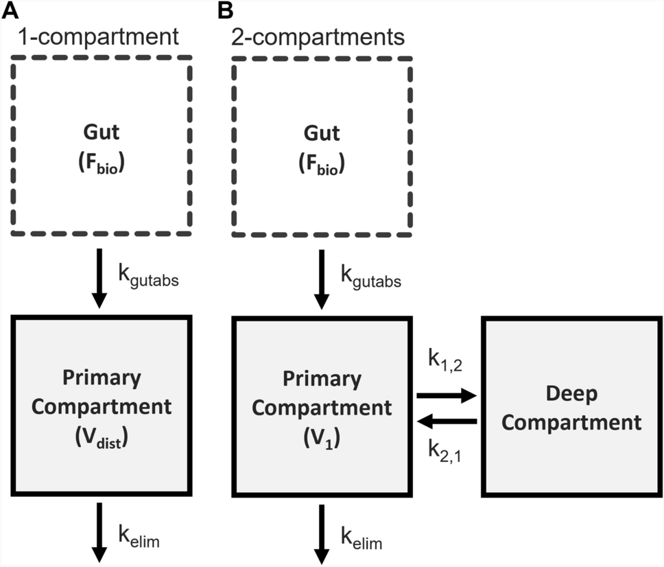
Step 1: hydrocortisone PK model refinement

The previously developed hydrocortisone PK model was a two-compartment disposition model that included a saturable absorption process of hydrocortisone, hydrocortisone binding to corticosteroid binding globulin and albumin and theory-based allometric scaling for volume and flow parameters [20]: Only the absorption process was re-evaluated and refined in this work. Two alternative more complex absorption models were evaluated, referred to as ABS1 (“split-dose”) model and ABS2 (“estimating number of transit compartments”) model, respectively. In the ABS1 model, the dose was split into two depot compartments, one with first-order absorption and one with transit compartments for absorption: The use of 2, 3, 4 and 5 transit compartments was evaluated. The fraction of dose being absorbed from the first depot compartment was estimated (FA), while the remaining fraction was absorbed from the second depot compartment (1-FA). The ABS2 model was a more commonly used transit compartment absorption model with estimated number of transit compartments [27]. The models ABS1 and ABS2 were developed and their performance compared. For both models, interindividual variability (IIV) models on absorption parameters were evaluated. Additionally, for the individuals from the first trial, interoccasion variability (IOV) models on absorption parameters were evaluated. Lastly, dose-dependencies on absorption parameters in both ABS1 and ABS2 models were explored.

Step 2: endogenous ACTH and cortisol model

To characterize ACTH time-dependent pulsatile secretion, surge functions were used in combination with a baseline secretion modeled by zero-order secretion plus first-order elimination. Surge functions (Eq. 1) are characterized by an amplitude (SA), width (SW), peak time (Pt) and an exponent (n) which dictates the shape of the resulting peak: The higher the exponent, the flatter the peak. The exponent n can only assume even positive values: 2, 4, 6 and 8 were evaluated. Pulsatile secretion models with two and three surge functions were evaluated.

$$S\left(t\right)=\frac\!\left/ \!\raisebox\right.\right)}^+1}$$

(1)

Interindividual variability was evaluated on all ACTH-related parameters before including cortisol data. Lastly, additive, proportional and combined residual unexplained variability (RUV) models were tested.

Cortisol production rate was assumed to depend exclusively on ACTH concentrations. For the ACTH concentration to cortisol production rate relationship linear, log-linear, Emax and sigmoidal Emax models were evaluated. For the quantitative characteristics of the cortisol distribution, protein binding and elimination processes, hydrocortisone PK EBEs were extracted from the most appropriate model from Step 1 and used as individual cortisol PK parameters in the development of the endogenous model. Then, the implementation of a feedback inhibition from cortisol unbound concentrations onto ACTH pulsatile secretion was evaluated using hyperbolic and sigmoidal Imax models. The negative feedback was assumed to be able to fully suppress ACTH pulsatile secretion. Similarly, DEX administration was implemented by fully suppressing ACTH pulsatile secretion in the trial periods when it was given, with and without hydrocortisone. Then, IIV was evaluated on cortisol production-related parameters as well as ACTH suppression-related parameters. Additive, proportional and combined RUV models were tested.

To evaluate the effect of body weight and age on all parameters on which IIV was included, a covariate analysis was performed by stepwise covariate modeling (SCM) using significance levels of 0.05 for forward inclusion and 0.005 for backward deletion: Linear, power and exponential relationships between covariates and parameters were evaluated.

Step 3: joint model parameters re-estimation

The developed endogenous ACTH and cortisol model from Step 2 and the refined hydrocortisone PK model from Step 1 were integrated into a single joint model. In this last step, all non-fixed parameters were re-estimated simultaneously.

Model evaluation

Intermediate models from Step 1 and Step 2 were evaluated based on parameter plausibility and precision, goodness of fit (GOF) plots and, if nested, compared based on the difference in objective function value (dOFV): For the comparison of the best ABS1 and ABS2 models Akaike information criterion was used (AIC) instead of OFV, since the models were not nested. The predictive performance of key intermediate models and the selected models from each step was also evaluated by visual predictive check (VPC, n = 1000). Additionally, the parameters precision of the selected models from each step was evaluated using sampling importance resampling (SIR).

Simulations: CAH patients and healthy individuals

To generate CAH patients with different extents of disease severity and to compare ACTH and cortisol concentrations in CAH and healthy state, the developed model from Step 3 was used to simulate (n = 1000) ACTH and cortisol concentration trajectories in 70 kg patients of different CAH severity and healthy individuals. CAH patients were simulated by assuming no (0% remaining enzymatic activity, severe CAH) or decreased (20% remaining enzymatic activity, mild CAH) endogenous cortisol production.

Simulations: Interaction with hydrocortisone therapy

The reduction in ACTH overproduction was used as a metric to evaluate optimal hydrocortisone dosing time in CAH patients with no endogenous cortisol production (severe CAH patients). In particular, ACTH overproduction was compared in severe CAH patients without hydrocortisone, and when 10 mg immediate-release hydrocortisone granules were given at 05:00 or 07:00.

Software

PsN (Perl Speaks NONMEM) v4.8.1 was used to access NONMEM v7.4.3 through Pirana v2.9.6 to perform modelling and simulation activities, while data management, data visualization and processing of modeling results were performed using R v4.2.1 with RStudio v2022.07.2 + 576.