Zebrafish

Fertilized zebrafish eggs, obtained from matings of heterozygous adults, were collected and cultured in 100 cm petri dishes at 28.5 °C with a 14 h:10 h light:dark cycle. All adult zebrafish and larvae were maintained in a fish facility overseen by the Aquatic Resources Program at Boston Children’s Hospital. Data on water quality, environmental conditions, diet, and other aspects of husbandry are available on protocols.io (https://doi.org/10.17504/protocols.io.br4mm8u6).

Birefringence assay

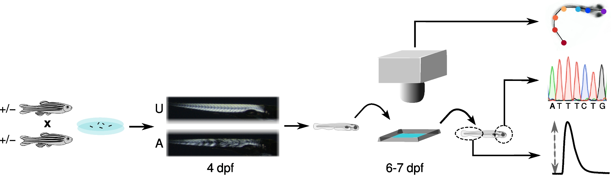
A non-lethal birefringence assay was used to classify larvae as affected or unaffected as previously described [19, 20]. Briefly, lightly anesthetized larvae were aligned between two glass polarizing filters, viewed with a stereo-microscope, and classified as unaffected if the tail and trunk musculature appeared bright and well-organized or affected of the muscle displayed gaps, breaks, or loss of birefringence. Affected and unaffected larvae were then transferred into 48 well plates, one larvae per well, and returned to the incubator until further study.

Experimental setup

Escape responses were evaluated in a rectangular arena formed by laser cutting a 20 mm × 30 mm opening in a 30 mm × 40 mm piece of acrylic. The arena was attached to the inside surface of a water-jacketed preparatory tissue dish (Radnoti, model 158,401) with aquarium grade silicon. Water from a temperature-controlled bath circulated through the jacket and beneath the arena. The arena contained fish water to a depth of ≈ 3 mm at the center in order to minimize movements in the z-plane. A micro thermocouple confirmed that the fish water temperature was maintained at 25 °C throughout data collection. An LED array and diffuser illuminated the arena from below.

Escape responses

A single larva was transferred into the arena and given 5 min to temperature equilibrate. Escape responses were elicited by a 1 ms electric field pulse [21] generated by a constant current muscle stimulator (Aurora Scientific, model 701) and delivered to platinum electrodes aligned along opposite walls of the arena. In preliminary studies, we established the current that consistently elicited an escape response and used this current for all subsequent trials.

Each larva was subjected to multiple trials until we had three acceptable escape responses (see quality control criteria below). A minimum of 60 s separated successive trials which is four times the inter-escape response period previously used to prevent habituation [12].

High speed videography

Videos (1280 × 864 pixels) were collected at 1000 frames/s using a monochrome high speed camera (Edgertronic SC2) positioned approximately 9 cm above the arena. A Nikon 50 mm f1.8D lens fitted with a 10X close-up lens produced a field of view that was roughly the same dimensions as the arena. Distance was calibrated each day of data collection and ranged from 44–45 pixels per mm.

A manually triggered, opto-isolated circuit was constructed to coordinate the escape response stimulus with the video recording. When triggered, the circuit opened the camera shutter but delayed the escape response stimulus by 10 ms producing 10 pre-stimulus frames for each video.

Markerless pose estimation

The open-source machine learning toolkit DeepLabCut (version 2.2rc3) was used to create a deep neural network for estimation of larval pose [22, 23]. To develop the neural network, we collected escape responses of 10 wild-type AB larvae (6 pdf). A kmeans algorithm selected 25 frames from each video that encompassed a diversity of poses. Each of the 250 frames were manually annotated with the following keypoints: TS, tip of the snout; S1, anterior aspect of the swim bladder; S2, posterior aspect of the swim bladder; T4 tip of trunk or tail; T2, point midway between S2 and T4; T3, point midway between T2 and T4; T1, point midway between S2 and T2. The keypoints defined six body segments: head, swim bladder, tail1, tail2, tail3, tail4. The keypoints were chosen so that we could quantify the length of the larva’s body, track its approximate center of mass, and model the curvature of its body.

The neural network was initially trained using ResNet50 architecture for 7.5 × 105 iterations using an 80% training to 20% testing split of the annotated dataset. Likelihood values were sometimes low during C-starts, when the tip of the tail was aligned very closely to, or even temporally occluded by, the head. To refine the network, we identified escape responses from six wild-type larvae where this occurred (3–8 frames per video). Keypoints with low likelihood scores (< 0.98) were either manually re-labeled or deleted (if occluded). These 28 newly annotated frames were merged with the original 250 annotated frames, the new data set was split into training (80%) and test (20%) sub-sets, and the neural network trained for 106 iterations.

Network training was conducted on a Dell Precision 3640 desktop computer (Intel Core i7-10700 K, 8 Core, 32 GB RAM, Ubuntu version 20.04 LTS) equipped with a NVIDIA GeForce RTX 3080 graphical processing unit. With this configuration, the 106 iterations used to train the neural network were completed in about 12 h. Escape response videos were analyzed on the same hardware, requiring about 5 s per trial. The DeepLabCut neural network developed for estimating larva pose from an escape response video is available at https://github.com/jjwidrick/danio-ER-DNN.

Kinematic analysis

Custom scripts written in R [24] were used to calculate morphological and kinematic variables from the DNN output. These scripts have been incorporated into an R package named “daniomotion” which is available at https://github.com/jjwidrick/daniomotion. Tail segment angle data were smoothed using locally estimated scatterplot smoothing (LOESS, span = 0.10) prior to analysis. Tail curvature was defined as the sum of the four individual trunk segment angles. Tail rotation direction was standardized between larvae by defining positive rotation as the direction of the first major bend of the tail (the C-start). Tail curvature angular velocity was calculated using the central finite difference equation [25]. The initiation of movement was determined as the post-stimulus frame where tail curvature exceeded the preceding frame by 2%.

Linear kinematics were based on the movement of the larva’s center of mass (COM). Larval COM is reported to fall at various locations between the anterior and posterior edges of the swim bladder [14, 15, 26, 27]. For the purposes of this study, we used keypoint S2 to represent the COM [14]. Distance was defined as the length between S2 on consecutive frames. Displacement was defined as the vector between S2 position at movement time zero and the current S2 position. Distance and displacement were calculated from unfiltered data.

The instantaneous speed of S2 was determined as the first derivative of distance with respect to time using the central difference method. The acceleration of S2 was determined as the second derivative of displacement with respect to time. Instantaneous speed oscillates due to the undulatory nature of swimming. In order to increase consistency in determining the exit speed from each stage as well as the overall peak instantaneous speed, the raw speed response was smoothed using LOESS (span = 0.7).

Linear kinematics were normalized to larval body length (BL). Body length was calculated as the sum of the 6 body segments, averaged across the pre-movement frames.

Stage-specific kinematics

We calculated performance variables that took into account the entire escape response (overall distance, displacement, peak instantaneous speed, and peak acceleration). We also partitioned the escape response into three stages [28] and determined stage specific kinematics. The first change in tail curvature sign delineated the transition from the stage 1 C-start to the stage 2 power stroke. The next change in sign indicated the end of the power stroke and the beginning of stage 3 burst swimming. Some larvae had a small counter tail bend that preceded the much larger C-start. These bends were ignored in analysis [29].

We used successive extremes in tail curvature to define a tail stroke (two sequential tail strokes equals one tail beat cycle). Stage 1 and 2 consist of single tail strokes. Stage 3 consists of multiple strokes and we choose to carry the stroke nomenclature through stage 3 rather than convert strokes to tail beats. The number of stage 3 tail strokes varied between larvae. Therefore, for stage 3 we calculated variables that encompassed the entire stage (total stage duration, total stage distance, total stage displacement, and average stage speed) as well as variables that were based on the number of full strokes completed by the larvae, ignoring any partial strokes at the end of the stage. These variables were the average number of tail strokes, the average distance covered/tail stroke, the average tail stroke peak to peak amplitude, and the average tail stroke frequency.

Muscle contractility

A subset of sapje strain larvae that had been subjected to ER analysis were subsequently used for assessment of muscle contractility as previously described [30]. Briefly, a larva was euthanized and one end of the tail was attached to the output tube of an isometric force transducer. Attachment was made at the gastrointestinal opening. This attachment point was easy to replicate as the 10–0 silk thread used for fastening the preparation was guided to this location by the notch formed at the intersection of the ventral and dorsal fin folds. This consistency in attachment enabled valid absolute force comparisons between preparations. The other end of the preparation was attached to an immobile titanium wire at a location that was approximately 2 mm distal to the GI opening.

Tail muscle preparations were studied in a bicarbonate buffer (equilibrated with 95% O2, 5% CO2) that was maintained at the same temperature as the escape response trials (25 °C). A muscle twitch was induced using a single supra-maximal square wave pulse, 200 µs in duration, that was delivered to platinum electrodes flanking the preparation. The length of the preparation was adjusted to maximize twitch force. Contraction time, half-relaxation time, and the maximal rates of tension development and relaxation were calculated from the peak twitch force records [30].

Genotyping

Larvae were euthanized after completion of their escape trials. Genomic DNA was extracted from the heads and used as a PCR template. The sapje and sapje-like primer sets have been previously described [31]. Sanger sequencing was conducted at the Molecular Genetics Core Facility at Boston Children’s Hospital.

Quality control

Raw videos were analyzed by the DNN without any pre-processing. Each escape response trial had to satisfy the following criteria in order to be included in further analysis. First, larvae had to remain stationary during the 10 ms pre-stimulus period. Second, the trial had to be accurately tracked by the neural network. Poor tracking was easily identified by a string of likelihood values < 0.98 coupled with erratic trunk curvature plots. Third, the video had to capture sufficient frames to enable us to analyze 60 ms of movement. Finally, only trials where there was agreement between fish phenotype (birefringence) and genotype (Sanger sequencing) were included in the final analysis, i.e. all affected fish genotyped as −/− and all unaffected fish as either +/+ or +/−.

Statistical analysis

We evaluated 678 escape responses recorded from 49 sapje mutants and 73 wild-type siblings (29 +/+, 44 +/−) and 51 sapje-like mutants and 53 wild-type siblings (16 +/+, 37 +/−). These larvae were obtained from 7 and 4 matings of groups of adult sapje and sapje-like fish, respectively. Approximately 40% of the sapje strain larvae were subsequently used in the muscle physiology experiments (11 +/+, 20 +/−, 17 −/−). Unless otherwise noted, all results are based on these sample sizes.

Point estimates of effect sizes and variability were calculated using a bias-corrected-and-accelerated bootstrap approach. Standardized effect sizes were calculated using Hedges’s g with bias-corrected-and-accelerated intervals. Both methods used 5000 resamples and 99% confidence intervals.

To classify mutant (−/−) and wild-type (+/+ and +/−) groups, we employed a random forest model. All variables, regardless of stages, were used for modeling. For constructing trees, 2/3 of the data were used for training, and the remaining data were used for the out-of-bag calculation. To identify the important variables, the means of GINI importance were measured. To validate the random forest model, we employed a linear support vector machine (SVM) model with various values of C (ranging from 0.00 to 5.00) to gain the most accurate model, allocating 70% of the data for training and 30% for testing. Our validation process included conducting a tenfold cross-validation.

Statistical analysis was conducted with R version 4.4.1 [24] and the following packages: bootES [32], factoextra [33], FactoMineR [34], randomForest [35], ROCR [36], e1071 [37], kernlab [38], ROCit [39].