Medical Imaging and Patient Data

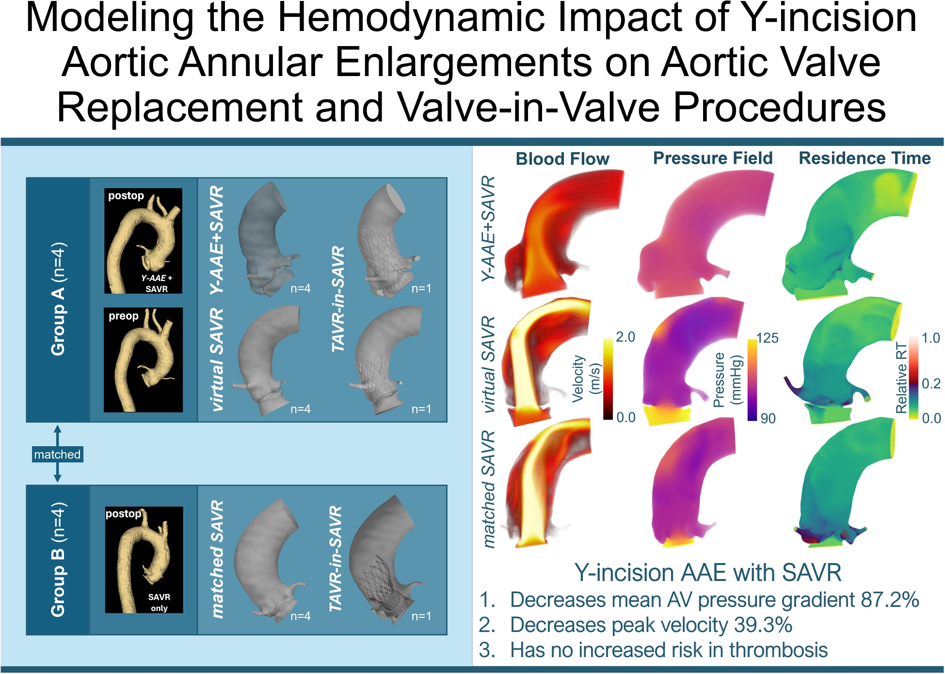
Fifteen distinct models (12 SAVR and 3 SAVR-in-TAVR) were generated. To form our patient cohort, we first reviewed patients undergoing first-time Magna Ease SAVR, with and without Y-AAE, at the University of Michigan Hospital. We included adult patients with severe aortic stenosis and normal aortic annulus size (19-25 mm) that had available pre- and post-operative CT images with contrast. We excluded patients with concomitant ascending/arch replacement (Table 1). From this list we identified 4 patients with SAVR and root enlargement (Y-AAE+SAVR). Pre-operative anatomies for these patients were used to virtually deploy a SAVR valve without enlargement (virtualAVR) as a control. In addition, each of the 4 Y-AAE+SAVR patients were paired to SAVR only patients (n\( = \)4, matchedSAVR) from the list that had similar age, sex, body surface area, ejection fraction, and native annulus diameter (Table S1). Finally, a collection of matched Y-AAE+SAVR, virtualSAVR and matchedSAVR were used to virtually deploy a TAVR to evaluate valve-in-valve hemodynamics. All patients had pre- and post-procedure CT images acquired on 64-detector CT scanners using helical acquisition mode (GE Medical System Discovery CT750 HD) with a spatial resolution of 0.3 to 0.7 mm. Images were acquired during intravenous iopamidol injection, using retrospective ECG-gating. Institutional review board approval was obtained (protocol No. HUM00211344), with no informed consent required.

Fig. 1

Modeling Pipeline and Model Generation: (A) Pre- and post-operative data acquisition, (B) segmentation of aortic root blood volume and SAVR, (C) model generation, and (D) CFD modeling where flow is prescribed at the inflow plane (green) during systole and pressure during diastole. Valve plane (blue) is open during systole and closed during diastole. SAVR valve leaflets (black), SAVR and TAVR stent (gray). A two-element Windkessel model is prescribed at the outflow plane (cyan), and volumetric flux is prescribed at the coronary arteries (magenta). (C) Model generation for the Y-AAE+AVR (row 1), virtualAVR (row 2), and matchedAVR (row 3). To that end, C1) data is acquired from two patients, and C2) segmented to generate C3) the final SAVR models. A virtual TAVR deployment is performed to generate TAVR-in-SAVR models (C4). (SAVR, surgical aortic valve replacement; TAVR, transcatheter aortic valve replacement; Y-AAE, Y-incision aortic annular enlargement)

Anatomic Reconstruction and Model Generation

We aimed to evaluate the hemodynamic impact of Y-AAE on SAVR procedures. This was achieved by reconstructing patient-specific anatomies from axial CT images and generating computational models (Fig. 1). The process began with the manual segmentation of CT images which were then converted into tetrahedral volume meshes with boundary layers using SimModeler software [14]. Each model had an average element side length of 1 mm and boundary layer edge length of 0.15 mm.

The model generation pipeline is illustrated in Fig. 1C. Post-operative CT images from a patient who underwent SAVR with Y-AAE (‘Patient A’) were used to create the Y-AAE+SAVR models (Fig. 1C, top row). Patient B, who underwent SAVR without Y-AAE, was selected as a control, matched to Patient A using parameters from Table S1 (matchedSAVR). Additionally, pre-operative CT images of Patient A were utilized to build an additional control model for comparison with the Y-AAE+SAVR. To generate this control, a Carpentier-Edwards PERIMOUNT Magna Ease aortic valve was virtually implanted into Patient A’s pre-operative anatomy (Fig. 1C5), creating a 3D anatomical model representing post-SAVR without Y-AAE (virtualAVR). A 3D model of the Magna Ease valve from the matchedSAVR patient (‘Patient B’; Fig. 1C, bottom row) was virtually implanted and subtracted from Patient A’s pre-operative 3D model, leaving only the blood volume for the virtualAVR.

To study the impact of Y-AAE in potential TAVR-in-SAVR, we virtually deployed (Fig. 1C6) a Medtronic CoreValve into the anatomies of Y-AAE+SAVR, virtualSAVR, and matchedSAVR (Group 3; see Fig. 1C4). To create the TAVR-in-SAVR models, a 3D model of a CoreValve was resized based on the primary implanted Magna Ease valve size and Medtronic guidelines [15]. Commissures of the two valves were aligned and the bottom of the CoreValve was positioned to be 4 mm below the bottom of the Magna Ease valve [16, 17]. The Magna Ease leaflets were held in an open configuration (Fig 1D, vTAVR).

Computational Fluid Dynamic Modeling

A stabilized form of Navier-Stokes equations was used to solve for the blood flow (pressure and velocity) in the different anatomies [18]. Blood was modeled as an incompressible, Newtonian fluid. To predict the flow, we utilize the finite-element-based solver \( \varvec} \) Heart to perform CFD simulations [19]. The pressure (p) and blood velocity (\( } \)) are determined by solving the Navier-Stokes equations within the given domain,\( \Omega \). These equations read:

$$\begin&\rho \frac}} + \rho } \cdot \nabla } - \nabla \cdot \varvec = \varvec, \,\qquad \qquad \qquad \text \Omega _t, \end$$

(1)

$$\begin&\nabla \cdot } = 0, \qquad \qquad \qquad \qquad \qquad \qquad \qquad \qquad \text \Omega _t, \end$$

(2)

$$\begin&\varvec \cdot \hat}} = \varvec_N, \qquad \qquad \qquad \qquad \qquad \qquad \qquad \quad \, \text \Gamma _t^N, \end$$

(3)

$$\begin&} = }}}_D, \qquad \qquad \qquad \qquad \qquad \qquad \qquad \qquad \quad \text \Gamma _t^D, \end$$

(4)

where \( \rho \)=1.026 g/ml is the fluid density, \( \varvec = \mu _f(\nabla } + \nabla }^T)+ p} \), is the Cauchy stress tensor, \( \Gamma \) is the boundary on \( \Omega \), and \( \mu _f \) =0.004 Pa\( \cdot \)s is the bulk fluid viscosity. A stabilization scheme proposed by Hoffmann et al. was applied allowing for \( \mathbb ^1-\mathbb ^1 \) elements to be used for fluid velocity and pressure without causing spurious oscillations [20].

The aorta was modeled as a rigid domain with no-slip conditions at the wall. The aortic valve was modeled as an orifice plane, opening and closing at the beginning and end of systole (Fig. 1D, blue) [21]. While this simplification neglects valvular dynamics, this approach models the “best-case scenario” as leaflet dynamics tend to increase maximal valvular velocity and increase mean TPG. To model the true aortic valve internal geometric orifice area (GOA), it was prescribed to be 6.0 mm less than the implanted valve’s internal diameter [22]. To isolate the impact of anatomy and facilitate comparisons across the cohort, we prescribed identical boundary conditions across all models. This included a heart rate of 70 bpm and a stroke volume of 73.5 mL with a prescribed flux during systole at the inflow plane and prescribed pressure during diastole (Fig. 1D). A volumetric flux was prescribed at the coronary arteries (Fig. 1D). After valve closure, a variable pressure was prescribed to mimic LV diastolic filling pressures. At the outflow plane, the 3D model was coupled to a 2-element Windkessel model to provide physiological pressure/flow boundary conditions (Fig. 1D) [23]. The Windkessel model had a resistance of 0.121 (Pa\( \cdot \)s)/mm\( ^3 \) and a compliance of 9.37 mm\( ^3/ \)(Pa\( \cdot \)s). Each problem was run for 3 cardiac cycles, with a time step of 0.0008 seconds, to reach convergence. This was determined where the peak velocity and mean TPG were within 5% cycle to cycle.

The Navier Stokes solution was then used to solve for regions of high flow recirculation which is correlated with increased thrombosis risk [24]. To evaluate this, we calculated the residence time. This quantity was calculated as a field, detailing the amount of time a fluid particle spends inside any region in the aortic root and ascending aorta. To solve for the time a fluid particle has been in the region of interest (\( \phi \)), for any t \( \in \) [0, T], we satisfy the following advection-diffusion equation [24]:

$$\begin&\partial _\phi +}\cdot \nabla \phi +\nabla \cdot }\nabla \phi =}, \,\qquad \qquad \qquad \text \Omega , \end$$

(5)

$$\begin&\phi = 0, \qquad \qquad \qquad \qquad \qquad \qquad \qquad \qquad \qquad \,\, \text \Gamma ^D, \end$$

(6)

$$\begin&}\nabla \phi \cdot \hat}}=0, \qquad \qquad \,\,\,\qquad \qquad \qquad \qquad \quad \quad \, \text \Gamma ^N, \end$$

(7)

where \( } \) is the predefined advective field solved from the Navier-Stokes equations and \( \phi \)=0 on the inflow and outflow faces (\( \Gamma ^D \)) with a Dirichlet boundary condition. The diffusivity (D) is set to 0 as it is assumed to have negligible impact. A constant source is added, making the field grow consistently with time, unless it is advected away and replaced by new fluid. We use the 3rd cycle solution from our fluids problem as the prescribed advective field. Each problem was run for 14 cardiac cycles so that there was less than a 5% change in model’s mean residence time. The field output was scaled by the total simulation time, T, which results in the relative RT field. This value varied from 0 to 1, where a value of 1 means that those blood particles do not leave the fluid volume, a value of 1/3 means it takes T/3 seconds for blood particles in that region to exit the domain, and a value of  0 means the blood particles leave the fluid volume nearly instantly.

Quantitative Analysis

To quantify the impact of Y-AAE+SAVR vs SAVR we evaluated the following variables of interest:

1.

Peak Velocity: This measure was calculated similar to echo measurements whereby we examined hemodynamics in the effective orifice area, taking the maximum velocity magnitude downstream of the aortic valve.

2.

Mean TPG: This was defined as the average positive pressure difference between the inlet plane and a plane 30 mm downstream of the aortic valve during forward flow.

3.

Relative RT (t/T): This was the amount of time (t) a particle has been in the 3D domain divided by the current time (T). We quantify the maximum and mean relative RT. To quantify if there are large volumes with high RT, we also evaluated the percentage volume that has a relative RT>0.2.