Data

To better understand how community-dwelling adults age, the Baltimore Longitudinal Study of Aging (BLSA) was established in 1958 [20]. We selected a subset of the research participants who underwent brain MRI scans and vestibular testing in the same study visit between 2013 and 2015 and were \(\ge\) 60 years old. From the total participant cohort, 103 individuals matched the criteria for our study subset. The group’s mean age (± SD) was 76.99 years (± 8.7), and 72% were males. All participants provided written informed consent and were cognitively healthy and diagnosed with no history of vestibular, ophthalmological, microvascular, or neurodegenerative disease. The BLSA study protocol (03-AG-0325) was approved by the National Institute of Environmental Health Sciences Institutional Review Board.

MRI Testing

The National Institute on Aging’s (NIA) Clinical Research Unit used a 3 T Philips Achieva scanner to conduct the MRI scans. Sequences included a T1-weighted volumetric scan magnetization prepared rapid acquisition with gradient echo (MPRAGE; TR = 6.5 ms, TE 3.1 ms, flip angle = 8°, 256 × 256 image matrix, 170 slices, voxel size = 1.0 × 1.0 mm, slice thickness = 1.2 mm, FOV = 256 × 240 mm). T1-weighted volumetric images were collected in the sagittal plane.

Vestibular Testing

Vestibular function testing includes the cVEMP test to assess saccular function, the oVEMP test to assess utricular function, and the video head impulse test (vHIT) which measures VOR gain to assess semicircular canal functioning. A vestibular-evoked myogenic potential (VEMP) is a short-latency potential that is evoked by activating vestibular receptors with sound or vibration. It is produced by electromyographic impulses that have been modified, either from the inferior oblique muscle for the ocular VEMP (oVEMP) or the sternocleidomastoid muscle for the cervical VEMP (cVEMP). The otolith organs appear to be the source of these reflexes and hence can be used to test the function of otolith organs [21, 22]. A commercial electromyographic system (software version 14.1; Carefusion Synergy, Dublin, OH, USA) was used for recording the VEMP signal. Electromyogram signals were recorded with disposable, self-adhesive, pre-gelled Ag/AgCl electrodes with 40-inch safety lead wires from GN Otometrics (Schaumburg, IL, USA). Electromyogram signals were amplified 2500 × and band-pass filtered, 20–2000 Hz for cervical vestibular-evoked myogenic potentials and 3–500 Hz for ocular vestibular-evoked myogenic potentials.

Both continuous and categorical measures were utilized for cVEMP, oVEMP, and VOR gain as independent variables of interest in separate analyses. For cVEMP and oVEMP, the continuous measure was the higher amplitude from either ear (corrected in the cVEMP case), and the categorical measure was a bilaterally absent response versus any present response. For VOR gain, continuous measures represented the average VOR gain from both eyes, whereas categorical measures classified responses as impaired (gain < 0.8) or unimpaired.

Cervical VEMP (cVEMP)

Participants laid with upper bodies increased at 30° from horizontal. A non-inverting electrode was placed at the mid-point of the sternocleidomastoid muscle, an inverting electrode was placed on the sternoclavicular junction, and a ground electrode was placed on the manubrium sterni. During stimulation and recording, participants were instructed to lift their heads from the headrest to provide tonic background sternocleidomastoid activity. A pre-stimulus rectified surface electromyogram signal of at least 30 µV was used required for accepting a cervical vestibular–evoked myogenic potential tracing [22]. Bursts of monoaural, 500 Hz, 125 dB sound stimuli were delivered using headphones (VIASYS Healthcare, Madison, WI, USA). The background EMG activity was obtained 10 ms before the start of the sound stimulus, and it was used to normalize the recorded myogenic potentials. In the analyses, the greater cVEMP from either ear was used. In accordance with established rules, an absent response was defined as one that fell below a threshold level. The assessment was then repeated to ensure accuracy [14, 16].

Ocular VEMP (oVEMP)

For ocular vestibular-evoked myogenic potential testing, participants laid with upper bodies increased at 30° from horizontal. A non-inverting electrode was placed on the cheek ≈3 mm below the eye, directly beneath the pupil, an inverting electrode was placed 2 cm below the non-inverting electrode, and a ground electrode was placed on the manubrium sterni. Before stimulation, participants were instructed to perform 20° vertical 19 saccades to ensure that symmetrical signals were recorded from both eyes. If signals showed > 25% asymmetry, the electrodes were removed, and new ones were applied. Participants were instructed to maintain a 20° up gaze during ocular vestibular-evoked myogenic potential stimulation and recording [22]. The midline of the face was tapped with a reflex hammer at the hairline and about one-third of the space between the inion and nasion. In this investigation, the best response from either ear was used. An absent answer was recorded and repeated for confirmation if the response fell below the predetermined threshold levels [21, 23].

VOR Gain Testing

The horizontal vestibular ocular reflex (VOR) was assessed using the video head impulse test (vHIT). The vHIT was performed in the plane of the right and left horizontal semicircular canals using the EyeSeeCam system (Interacoustics, Eden Prairie, MN, USA). The patient’s head was pitched down 30° to place the horizontal canals in the plane of stimulation, and subjects were asked to fix their gaze on a wall target about 1.5 m away. The head was moved at a small amplitude (approximately 5–15°) with high velocity (typically 150–250°/s) horizontally toward the right and left side at least 10 times in both directions. The direction of the head movement was randomized to be unpredictable. The EyeSeeCam system measured eye velocity and head velocity, and a corresponding VOR gain was calculated by dividing the eye velocity by the head velocity. A normal, compensatory VOR gain should equal 1.0. VOR gains less than 0.8, along with compensatory refixation saccades, suggesting a loss of peripheral vestibular function [23].

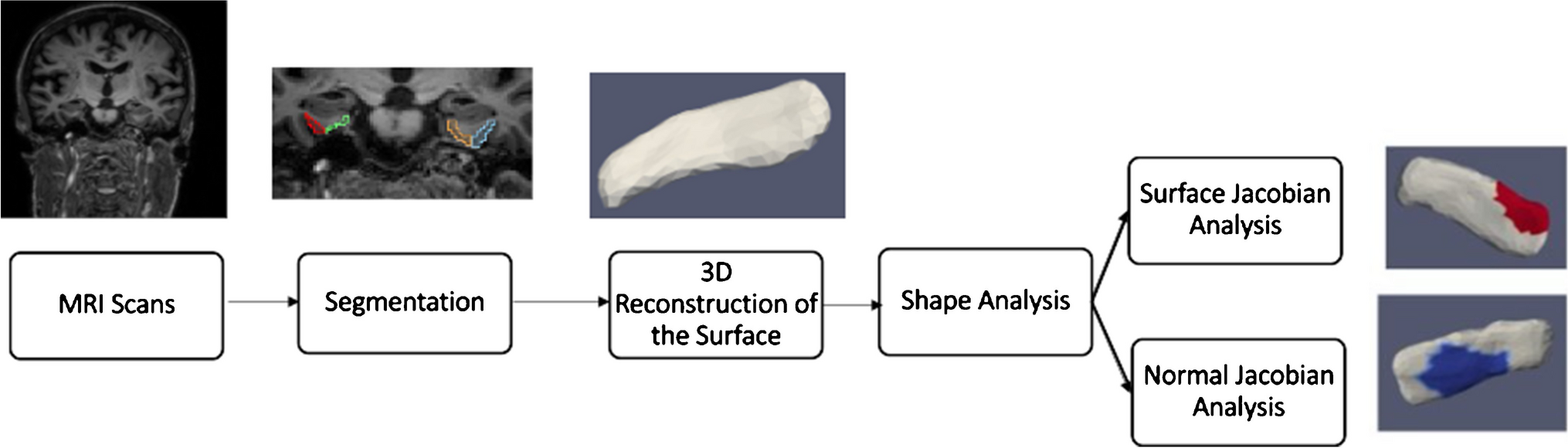
Pipeline

The general outline for shape analysis is shown in Fig. 1. A binary segmentation volume is created by segmenting the structure of interest from the brain’s MRI scans. A 3D surface is then obtained by triangulating the binary volume. Shape descriptors were determined by measuring how far each subject’s shape deviated from the population template. Regression is employed in statistical analysis, with shape descriptors as the dependent variable and vestibular factors as the independent variables. The following subsections go into further detail about each phase.

Fig. 1Segmentation and 3D Reconstruction of Surfaces

T1 scans were automatically segmented by registering them to multiple atlases using large deformation diffeomorphic metric mapping (LDDMM) [24]. The parcellation of the scans was based on the multiple-atlas likelihood fusion (MALF) algorithm [25, 26], with 286 defined structures. The parcellation was done through MRICloud, an online neuroinformatics platform that provides tools for automatic brain parcellation and surface registration (https://www.mricloud.org/). Surfaces were created from the binary segmentations using restricted Delaunay triangulation [27,28,29]. Since the accuracy of the segmentations and the surface reconstruction were crucial to the outcomes, quality control was carried out at every step, and manual editing of segmentations and surface meshes was done when necessary.

Shape Analysis

For shape analysis, the population of surface meshes was rigidly aligned and used to create a “mean shape” called the template. Templates were made separately for each structure’s left and right sides. The generated template is label- and group-blind and serves as a coordinate system for the population average. Each subject surface was registered to this template, first rigidly and then using surface LDDMM. The algorithm computes a smooth invertible mapping of the triangulated surface template onto the target surfaces. MRICloud provides the public with access to this pipeline [30, 31]. The MRICloud diffeomorphic registration pipeline yields two deformation values per vertex: Jacobian determinant of the 3D surface transformation and the surface Jacobian. The Jacobian determinant is a scalar that describes the volume change due to the diffeomorphic change of coordinates. The surface Jacobian is a scalar that describes the ratio between the surface area of the faces attached to a vertex before the transformation (i.e., the surface template) and following it (i.e., the surface template mapped to the target surface). Because surface shape can vary independently in terms of expansion/compression tangent to the surface (i.e., surface area change) and expansion/compression normal to the surface, we compute a third shape descriptor called the normal Jacobian. The normal Jacobian is the ratio between the Jacobian determinant and the surface Jacobian signifies the ratio between the length of an infinitesimal line oriented normally to the surface before and after the transformation. We analyze the surface and normal log-Jacobians independently. A positive (negative) surface log-Jacobian value denotes an expansion (contraction) of the template around that vertex in the direction tangent to the surface to fit the subject. Similarly, a positive (negative) normal Jacobian value denotes an expansion (contraction) of the template around that vertex in the direction normal to the surface to fit the subject. We fit the statistical model to each vertex, thus giving \(N\) models for each subject, where \(N\) is the number of vertices in the population template. The null hypothesis is:

$$_: \text= _}\text+ _}\text+_}\text+ _$$

The alternate hypothesis is:

$$_}:\text= _}\text+_}\text+ _}\text+_}\text+ _$$

where \(\text\) refers to the vestibular variables investigated (cVEMP, oVEMP, VOR Gain) and \(\text\) (intracranial volume) refers to the total volume within the skull, including left and right hemispheres, brain stem, cerebellum, and CSF (cerebral spinal fluid); therefore, \(\text\) reflects the head size. For each participant, Age in years is a continuous variable and sex is a binary variable, coded 1 for female and 0 for male. The unknown coefficients are \(\_}, _}, _}, _}\}\) for vestibular variables, and \(\text\), age, sex, and \(_\) are the constant terms estimated using least squares. The left and right brain structures are analyzed separately. The schematic of the procedure is shown in Fig. 2.

Fig. 2

Schematic of shape analysis

We use spectral clustering to partition all vertices (\(N\) ≈ 400) into \(k\) (6 to 7) clusters to boost the analytical power and limit the number of models being evaluated simultaneously [32]. Only the shape’s surface geometry is used in this procedure. Each segment’s maximal surface Jacobian is assigned to that cluster, resulting in \(k\) super-vertices [19]. In Fig. 7, each colored region represents one cluster, thus reducing the number of models from \(N\) (number of vertices, ≈ 400) to \(k\, a\) (number of clusters, 6 to 7). Permutation testing is used to calculate significance level or p-value to avoid multiple hypothesis problems (see the “Multiple Hypothesis Testing” section). The relative difference was expressed in terms of presence/absence when the categorical form of vestibular variables was used. In the case of continuous form, we report the relative difference with a 1 SD increase in cVEMP, as mentioned above. For completeness, we report our results from our investigation of the relationship between cVEMP and ERC and TEC surface Jacobians which was also investigated in a previous study of the same cohort [19].

Multiple Hypothesis Testing

The problem of multiple hypothesis testing arises from fitting a linear model to each cluster. The probability of making at least one type I error is significantly higher than alpha if the same procedure is applied to several hypotheses tested simultaneously, particularly when the number of hypotheses is large. Here we use permutation testing to control the family-wise error rate (FWER). Permutation tests build an empirical estimate of the distribution of the test statistic under the null hypothesis by permuting/resampling data. The test statistic from the real data is then compared to this distribution, and the p-value is the fraction of the population greater than the real test statistic. Here, the test statistic was chosen as a ratio of maximum square errors in the null hypothesis to maximum square error in the alternate hypothesis.

High-Field Atlasing

We used a high-field strength (11 T) MRI to label structures of interest on the MRI images used in this study as a posteriori. To help us define boundaries for our measurements of the ERC, we used the partitions established by Krimer et al. [33]. The Krimer partition, as it has been referred to throughout this study, divides the ERC into nine sub-regions. Established protocols were used to construct the lateral to medial coordinates for the 9 subregions [33,34,35]. This study defines the following 7 Krimer regions together as the ERC: (1) intermediate superior (ERC-Is), (2) intermediate rostral (ERC-Ir), (3) intermediate caudal (ERC-Ic), (4) pro-rhinal (ERC-Pr), (5) medial rostral (ERC-Mr), (6) medial caudal (ERC-Mc), and (7) lateral (ERC-L). This definition corresponds well with how the ERC is typically defined for most MRI studies. We represent the Krimer sulcal (ERC-S) and trans entorhinal regions, which correspond to the 8th and 9th Krimer atlas regions, together as the TEC [16, 18]. To assign Krimer labels to the population template, we first rigidly aligned the population template and the high-field atlas, and then we used surface LDDMM to map the population template onto the high-field atlas. Krimer labels were transferred to the population template vertices using the deformation field followed by a nearest-neighbor label assignment. Figure 3 shows the ERC population template with Krimer subfields. In a prior study, Kulason et al. (2020) highlighted the discrepancies stemming from different nomenclature about the TEC and ERC. Their comparative examination of four atlases provided insight into these disparities, with Fig. 4 in the paper as a reference point.

Fig. 3

View of ERC overlayed with Krimer partitions

Fig. 4

ERC template showing significant results for the clustered left and right sides of the ERC (view from the caudal end, upside-down) for categorical cVEMP