2.1 Study Population, Dosing, and Sampling Schedule

Combined data from HP and patients from 12 clinical trials between December 2014 and July 2021 were included (Table S1 of the Electronic Supplementary Material [ESM]): data from seven phase I studies in HP and organ impairment and five phase II/III studies in patients with RA, UC, AA, and vitiligo (NCT02309827, NCT02684760, NCT02958865, NCT02969044, NCT03232905, NCT03732807, NCT04016077, NCT03715829, NCT04037865, NCT04004663, NCT04634565, NCT02974868). Ritlecitinib dosing ranged from 5 to 800 mg/day. Details for dosing and plasma sampling are shown in Table S1 of the ESM. The study protocols were approved by the institutional review boards/ethics committees of the study sites and all participants provided written informed consent. The studies were conducted in compliance with the ethical principles originating in or derived from the Declaration of Helsinki and conducted according to the International Conference on Harmonization Guidelines for Good Clinical Practice.

2.2 Analytical Methods

Plasma concentrations of ritlecitinib were determined using validated, sensitive, and specific liquid chromatography-tandem mass spectrometric methods at York Bioanalytical Solutions and Covance Bioanalytical Laboratories (Shanghai, China). The lower limit of quantification for each study is shown in Table S1 of the ESM. Individuals who did not receive one or more doses of ritlecitinib or did not have one or more measurable concentration of ritlecitinib were excluded. No data imputations for missing or below the lower limit of quantification (BLQ) concentrations of ritlecitinib were performed. Sampled concentrations that were BLQ were excluded only during parameter estimation for all three iterations of population PK model development. Below the lower limit of quantification observations were available to assess model performance at representing the proportion of observations BLQ over time.

2.3 Base Model Development

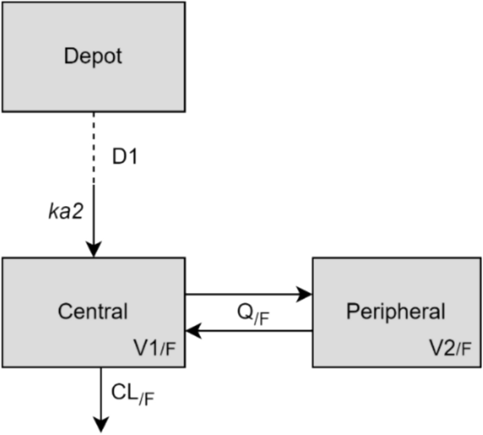
One- and two-compartment disposition models with first-order oral absorption were evaluated as candidate structural models. Time- and/or concentration-dependent changes in clearance (CL) and F such as Michaelis–Menten elimination kinetics, and direct or indirect response models for autoinhibition were explored for their ability to describe non-linearity in ritlecitinib pharmacokinetics.

Structural covariates known to be highly influential a priori were built into the structural model. For example, allometric scaling on PK parameters using body weight (exponents of 0.75 and 1 for CL and volume parameters, respectively, referenced to 70 kg), effect of inflammatory disease burden on ritlecitinib CL (consistent with observations made with other Janus kinase inhibitors), and dose, formulation, and high-fat meal effects on absorption parameters [9,10,11,12,13].

Inter-individual variability (IIV) was added to structural model parameters to account for differences between individuals in the population and was assumed to be log-normally distributed:

$$P_ = \theta_ \cdot e^ }} ,$$

(1)

where \(_\) is the individual value for parameter (P) in the ith participant, \(_\) is the population typical value for parameter P, and η is an independent random variable describing the variability in P among subjects with a mean of 0 and variance, ω2. Models with and without covariance between random effects were investigated.

A residual error model with a combination of additive and proportional effects was used to describe random unexplained variability (RUV) in ritlecitinib concentrations:

$$C_ = \hat_ + \sigma \cdot \varepsilon_ $$

(2)

$$\sigma = \sqrt _^ \cdot \sigma_^ + \sigma_^ } $$

(3)

where \(_\) is the ritlecitinib concentration in the ith participant, at observation j, \(\hat_\) is the model-predicted ritlecitinib concentration, \(\varepsilon_\) is a normally distributed random variable with a mean of 0 and variance of 1, \(\sigma_^\) and \(\sigma_^\) are the estimated variance of proportional and additive error, respectively. Structural model selection was guided by changes in the Akaike information criterion, standard goodness-of-fit diagnostic plots, precision of parameter estimates, and η-shrinkage.

2.4 Updated Model Development

Model parameters of the base model were re-estimated using a combined dataset of previous and new data to provide a reference structural model for stepwise covariate modeling.

2.4.1 Covariate Model Descriptions

The effect of a categorical covariate on a parameter was represented as a discrete relationship proportional to the population parameter. For example, the effect of patient type (PTST) on a parameter (P) was described as:

$$} = \left\l} 1 \hfill & }\;}\;\;}\;}} \hfill \\ }}} } \hfill & }\;}\;\;}\;}\;}} \hfill \\ \end } \right.$$

(4)

$$P_ = \theta_ \cdot e^ }} \cdot }$$

(5)

where \(\theta_}}}\) is the estimable parameter for the effect of patient type on P.

The effect of a continuous covariate on a parameter was represented as a power model referenced to the median of the observed data. For example, the effect of age (AGE) on P was described as:

$$P_ = \theta_ \cdot e^ }} \cdot \left( }_ }}}_}}} }}} \right)^}}} }} ,$$

(6)

where \(}_\) is the age (years) in the ith participant, \(}_}}}\) is the median age in the observed population, and \(\theta_}}}\) is the estimable parameter for the effect of age on P.

2.4.2 Covariate Selection

Stepwise covariate modeling approaches were conducted during the development of the updated model, and were used to identify key intrinsic and extrinsic factors that explained differences in ritlecitinib pharmacokinetics between individuals. Covariates for analysis included sex, age, baseline creatinine CL (Cockcroft–Gault), race, moderate hepatic impairment (based on Child–Pugh score), and formulation (tablets, capsules). Covariates were screened for a pairwise correlation. If a strong correlation existed, the more clinically relevant covariate continued to further analyses. Candidate covariates from screening procedures were independently added to the structural model to evaluate their individual significance in improving the fit of the model to the observed data. All covariates shown to be important from the univariable analyses were carried forward to the multivariable analyses.

In univariable analyses, the effect of incorporating an additional covariate parameter compared with the structural model was assessed by the likelihood ratio test. The covariate model was considered significantly better than the structural model if p < 0.01. Candidate covariates also had to satisfy additional criteria: (1) 95% confidence interval (CI) of the covariate parameter estimate did not include zero; (2) addition of the covariate results in a reduction in IIV on the target population parameter; and (3) model diagnostic plots showed an improvement.

In multivariable analyses, the covariates identified in univariable analyses were added sequentially to the structural model in order of statistical significance to form the full model. The sequential addition of a covariate to the model had to continue to fulfill the requirements described by univariable analyses. Selection of the final model was conducted by backward elimination of covariates from the full model in order of highest to lowest p-values, where a covariate remained in the model if its removal resulted in a significant increase in objective function value as assessed by the likelihood ratio test (p < 0.001).

2.5 Final Model Development2.5.1 Externally Evaluating the Updated Model

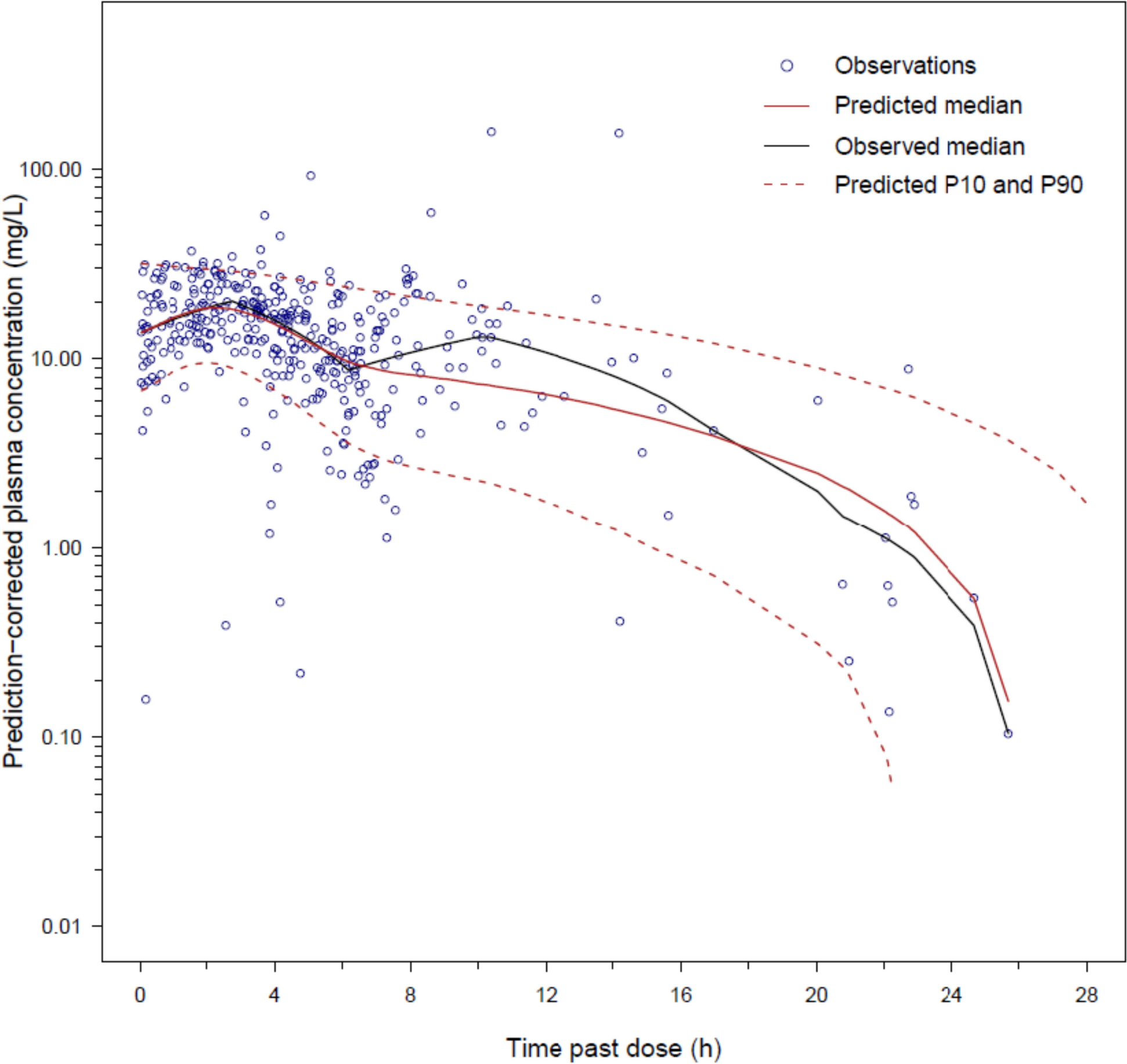
An external evaluation of the updated model was conducted to evaluate its ability to represent ritlecitinib concentrations available in an evaluation dataset (analysis population for the final model) before estimating population parameters. A combination of simulation-based (visual predictive check [VPC], prediction-corrected VPC, and assessment of normality of normalized prediction distribution errors) and empirical Bayes estimate (EBE)-based diagnostics (goodness-of-fit diagnostics and assessment of normality of conditional weighted residuals) were used. Model misspecification identified from this exercise guided covariate analysis of the final model. The structure of the updated model was not re-evaluated.

2.5.2 Frequentist Prior Update

The updated model was used as a “frequentist prior” (termed by Gisleskog et al. [14]) and the foundation of covariate analyses following external evaluation procedures. The PRIOR subroutine in NONMEM® applies a frequentist prior approach to inform population parameter estimates as opposed to fixing them. Here, a penalty is placed on the maximum likelihood (i.e., the objective function value), which accounts for the deviation of current model parameters from their prior estimate. This approach aims to reduce bias in parameter estimates where the reference population may be slightly different from the previous population used to develop the prior model [15].

The evaluation dataset for the final model predominantly consisted of sparse data from the phase II/III study in patients with AA (Table S1 of the ESM), such that it was anticipated that informative priors for all structural parameters adopted from the updated model were required to ensure adequate estimation of final model parameters. The final parameter estimates of the updated model were used as the prior during development of the final model and estimating parameters based on the evaluation dataset. The prior distributions of fixed-effect and random-effect (i.e., IIV) parameters from the updated model were assumed to be normally and normal-inverse Wishart distributed, respectively. Initially, the weight of priors on original model parameters were highly informative with low uncertainty (i.e., 10% relative standard error for the prior). Scenarios where fixed-effect parameters were uninformative (variance of parameter estimates set to 10,000) or highly informative (derived from the updated model’s variance-covariance matrix for parameter estimates) were examined. Scenarios where the prior variance of random-effect parameters for IIV were uninformative (dimensions of the variance-covariance matrix for IIV plus 1) or highly informative (dependent on the number of individuals used to build the prior model) were also examined [15]. Parameters quantifying the standard deviation of RUV and new covariates for assessment (such as age, severe renal impairment, and alopecia disease severity) did not include any prior information. The decision to proceed with a set of prior model parameters was based on model convergence (including successful minimization status), interpretation of final parameter estimates (i.e., consistent with expectations of the pharmacokinetics of ritlecitinib), and standard goodness-of-fit diagnostics.

2.6 Evaluation of Model Predictive Performance

The predictive performances of all models (base, updated, and final) were evaluated by VPCs stratified by candidate covariates and dose (not presented) and prediction-corrected VPCs based on 1000 simulations of their respective index datasets. The models’ abilities to adequately represent the observed proportion of BLQ concentrations were also evaluated.

2.7 Simulation Analyses for Evaluating the Impact of Covariates

Simulations were conducted to compare steady-state maximum plasma drug concentration (Cmax) and area under the concentration–time curve for the dosing interval (AUCτ) for ritlecitinib 50 mg once daily (QD) for 14 days for a series of covariate scenarios based on covariate effects in the updated and final models. The reference scenario was based on an HP, body weight 70 kg, fasted status, and administered the tablet formulation. For each covariate scenario, concentration–time profiles for 1000 trials of 118 randomly drawn individuals administered 50 mg QD for 14 days were simulated using the updated or final models and summarized by Cmax and AUCτ at steady state. The geometric mean ratios of Cmax or AUCτ for each covariate compared with the reference scenario were calculated for each trial.

2.8 Simulation Analyses for Assessment of Dose Proportionality and Accumulation

Simulations were conducted to compare steady-state Cmax and AUCτ for ritlecitinib 50 mg QD for 14 days versus (1) single ritlecitinib 50-mg dose Cmax and area under the concentration–time curve from time 0 to infinity (AUC0–∞), and (2) steady-state metrics for ritlecitinib 5–800 mg QD for 14 days for patients with AA with a body weight of 70 kg. For each dose scenario, concentration–time profiles for 1000 trials of 118 randomly drawn individuals administered ritlecitinib were simulated using the final model and summarized by Cmax and AUCτ on day 14 (or AUC0–∞ for a single-dose scenario). The geometric mean ratios of Cmax or AUCτ/AUC0–∞ for each dose scenario compared with the reference scenario were calculated for each trial. A steady-state accumulation ratio was assessed as the ratio of AUCτ divided by AUC0–∞.

2.9 Software

NONMEM version VII, level 4.3 (ICON Development Solutions, Ellicott City, MD, USA) was used for development of the base and updated models. NONMEM version VII, level 5.0 (ICON Development Solutions) was used for the development of the final model. In all models, parameter estimation used the first-order conditional estimation method with interaction algorithm and individual parameters were obtained from EBE. The ADVAN13 subroutine with TOL = 9 was used. Statistical and graphical output were generated using the R programming and statistical language (R version 3.6.1) [16].