
Remember me

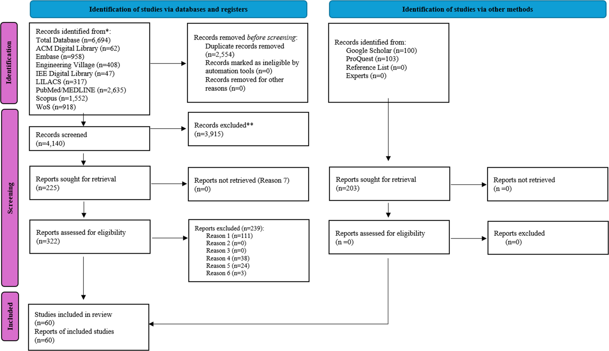
This study analyzed overnight PSG recordings from 257 healthy individuals and 382 insomnia patients, totaling 639 subjects recruited at Taipei Medical University (TMU) between 2015 and 2018. Healthy subjects were defined as having sleep efficiency (SE) \(\ge\) 85%, while insomnia patients had SE < 85%. All participants had no history of drug or alcohol abuse, nor neurological, psychiatric, or other sleep disorders. The insomnia group comprised subjects experiencing symptoms more than three times per week for at least one month, with significant impact on daily life. Insomnia diagnosis required: (1) SE < 85%, (2) sleep onset time (SOT) > 15 minutes, and/or (3) wake after sleep onset (WASO) > 30 minutes [7]. The sample was stratified by age groups: 0-29 years (n=62), 30-44 years (n=217), 45-64 years (n=282), and 65+ years (n=78), with complete demographic details in Table 1. The study was approved by the Institutional Review Board of TMU. All participants refrained from medication use and limited caffeine intake before the study. Overnight PSGs were recorded using a Siesta 802 system, comprising two EEG channels (C3-M2, C4-M1), a single EOG channel (ROC-LOC), and chin EMG. Signals were digitized at 256 Hz (16-bit resolution) and scored according to AASM guidelines [7]. Table 2 summarizes sleep stage distributions and key indices for both groups.
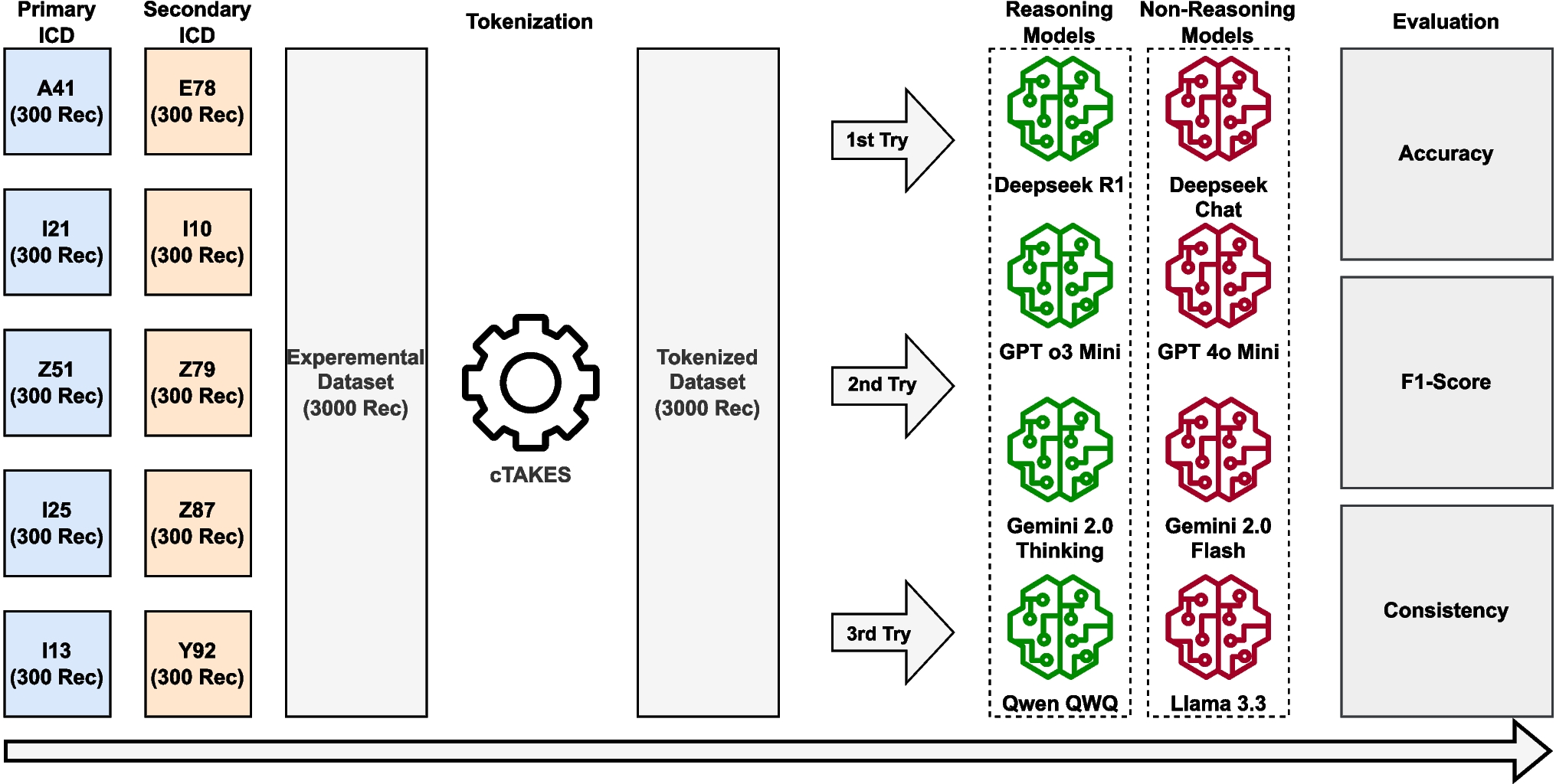
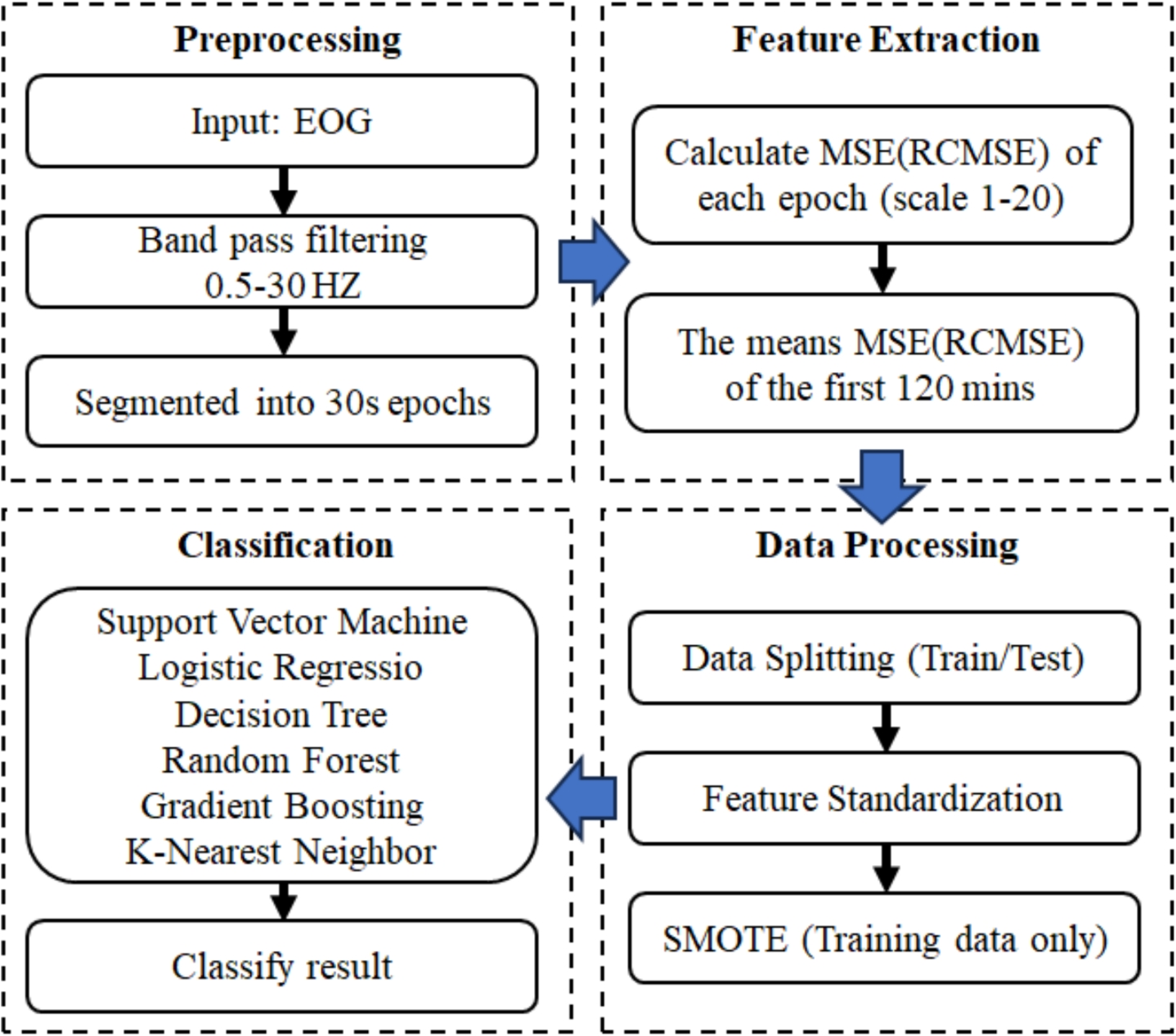
Table 1 Statistics and demographic distribution of the TMU Sleep Research Dataset (2015–2018) by age groupTable 2 Summary of sleep stage distributions and sleep-related indices for healthy and insomnia groups2.2 MethodsFigure 1 illustrates the proposed short-time insomnia detection system using single-channel EOG with MSE and RCMSE analysis, comprising four stages: signal preprocessing, feature extraction, data processing, and classification.
Fig. 1
EOG-based insomnia detection framework. Four-stage process: signal preprocessing, feature extraction, data processing (splitting/standardization/SMOTE), and classification with multiple algorithms
2.2.1 PreprocessingRaw EOG signals were filtered with an eighth-order Butterworth band-pass filter (0.5–30 Hz) and segmented into 30-second epochs per AASM guidelines [7].
2.2.2 Feature extractionMultiscale Entropy (MSE) MSE extends entropy analysis to multiple time scales, providing a comprehensive measure of signal complexity. Given an EOG time series with N samples, \(x = \\), and scale factor \(\tau\), the coarse-grained series \(y_(j)\) is calculated as:
$$\begin y_(j) = \frac\sum _^ x_i, \qquad 1 \le j \le \frac. \end$$
(1)
For each scale factor \(\tau\), sample entropy is computed on the corresponding coarse-grained series. Thus, MSE at scale \(\tau\) is defined as:
$$\begin \textrm(\tau ) = \textrm(r, m, y_). \end$$
(2)
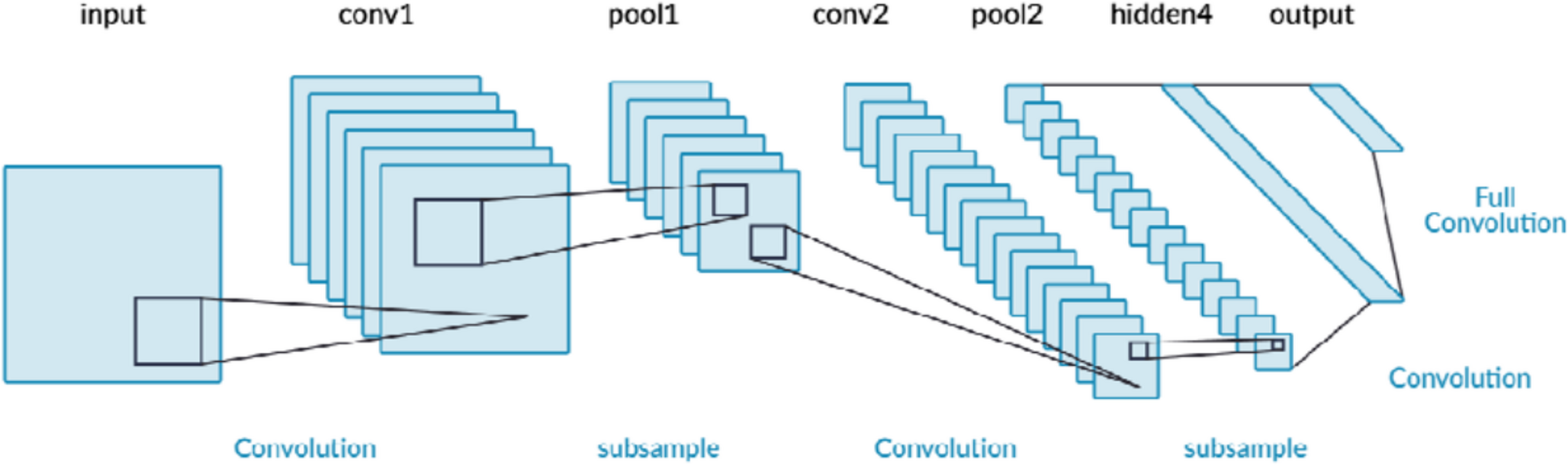
Refined Composite Multiscale Entropy (RCMSE) RCMSE addresses MSE’s limitation of increased variability at larger scale factors by generating multiple coarse-grained series for each scale, as illustrated in Fig. 2. For scale factor \(\tau\), the j-th element of the k-th coarse-grained series is:
$$\begin y^_k(j) = \frac\sum _^ x_i, \quad 1 \le j \le \frac,\ 1 \le k \le \tau . \end$$
(3)
RCMSE at scale \(\tau\) is then defined as:
$$\begin \textrm(\tau ) = -\ln \left[ \frac\sum _^ C^_(r)}\sum _^ C^_(r)} \right] . \end$$
(4)
Fig. 2
Illustration of the coarse-graining process in MSE/RCMSE analysis: scale factor 2 (upper panel) averages pairs of data points, while scale factor 3 (lower panel) averages groups of three points
Feature Construction Both MSE and RCMSE were calculated for each 30-second EOG epoch using scale factors 1-20. To assess different sleep durations on insomnia detection, we computed mean entropy values for cumulative durations (5-120 minutes in 5-minute increments). For each subject, entropy values were averaged over cumulative time windows using:
$$\begin \overline_ = \frac \sum _^ f_ \end$$
(5)
where \(f_\) is the entropy value of the k-th epoch at scale i (1-20), and j represents epoch count from 10 to 240 in steps of 10 (5-120 minutes). Each time window yielded feature sets \(\_, \overline_, \ldots , \overline_\}\) per subject.
2.2.3 Data processingFeatures were processed through a three-step pipeline: (1) random subject partitioning into training (80%) and testing (20%) groups; (2) z-score normalization with parameters calculated solely from training data; and (3) SMOTE [24] application to address class imbalance. For comprehensive evaluation, we examined all combinations of 20 scale factors and 24 time windows across 10 independent validation rounds with different random subject assignments.
2.2.4 ClassificationSix classifiers suitable for microcontroller implementation were evaluated: Support Vector Machine with polynomial kernel (degree=3, C=1.0), Logistic Regression with LBFGS solver, Decision Tree with maximum depth of 4, Random Forest with 200 estimators and 16 maximum leaf nodes, Gradient Boosting Classifier with default parameters, and k-Nearest Neighbors (k=5, Euclidean distance). All were implemented using scikit-learn with fixed random seed (42) where applicable.
2.3 Evaluation metricsPerformance was assessed using accuracy, sensitivity, specificity, F1 score, and Cohen’s kappa coefficient (\(\kappa\)) [25]. These metrics are defined as:
$$\begin \text &= \frac \end$$
(6)
$$\begin \text &= \frac \end$$
(7)
$$\begin \text &= \frac \end$$
(8)
$$\begin \text _1&= 2 \times \frac \times \text } + \text } \end$$
(9)
$$\begin \kappa&= \frac \end$$
(10)
where TP, TN, FP, and FN denote true positives, true negatives, false positives, and false negatives, respectively. Cohen’s kappa quantifies agreement between the proposed method and expert annotations, correcting for agreement expected by chance.
Comments (0)