Study design

Our study is a retrospective study in which the data collection was considered before the performance of index tests and reference standards. It is considered a diagnostic accuracy study because the accuracy of a newly developed deep learning model (DLM) in the automatic detection and segmentation of the MB2 canal in maxillary first molars is assessed by comparison with the opinion of the experienced radiologists, which represents the ground truth and its results are represented in the form of accuracy, sensitivity (recall), positive predictive value (precision) and receiver operating curve. In accordance with the code of ethics, this study was undertaken after the approval of the Research Ethics Committee of the Faculty of Dentistry, Cairo University. on 25/1/2022, and it complies with the Declaration of Helsinki (2013).

Patient declaration of consent was obtained via a Helsinki declaration consent form in their native language (Arabic). Provided is the English version of said form and a signed Arabic one by one of the study participant.

Sample size calculation

A power analysis was conducted to ensure sufficient power for a two-sided statistical test of the null hypothesis that the accuracy of the DL model is equivalent to that of the radiologist’s opinion. A 95% confidence interval and a specificity value of 88.0% were used for the DL group, as derived from a prior study [38], alongside a 100% specificity for the ground truth.

The sample size calculation was approved by the Medical Biostatistics Unit, Faculty of Dentistry, Cairo University, on 17/1/2022.

Radiographic dataset

The CBCT scans used in this study were obtained from the CBCT database available at the department of Oral and Maxillofacial Radiology, Faculty of Dentistry, Cairo University, Cairo, Egypt. The scans were obtained as a part of the diagnosis and treatment planning of the included patients.

All the selected scans were acquired using a voxel size of no more than 0.075 mm and featuring fully erupted maxillary first molars with complete root formation. Exclusions comprised maxillary first molars exhibiting developmental anomalies, external or internal root resorption, root canal calcification, prior root canal treatment, post-restoration, or root caries. Additionally, CBCT images of suboptimal quality, those with significant scattered artifacts hindering accurate assessment, as well as scans with a field of view (FOV) extending beyond a single arch or employing a voxel size exceeding 0.075 mm, were also excluded.

All the included scans (37 scans) were taken via a Planmeca Promax 3D MID CBCT machine, and the imaging protocol was standardized as follows: exposure parameters: 87 KVp, 8 mA, exposure time 12 s; voxel size 0.075 mm; and FOV 5 × 5-5 × 8 cm. Thirty-seven maxillary molars with MB2 canals (n = 20) and without MB2 canals (n = 17) were included.

Radiographic annotation (ground truth)

CBCT scans were imported into 3D slicer software program (open-source free software version 5.2.2, Harvard University, USA) for data annotation, which was performed in 2 separate steps: (classification and segmentation).

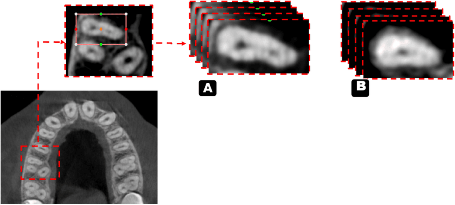
Regarding the classification stage, radiologist-dependent MB2 canal detection was performed on axial cuts along the entire length of the root and then classified into the presence or absence of the MB2 canal, which was confirmed and agreed upon by 2 oral and maxillofacial radiologists (OMFRs) (8 & 15 years of experience) (Fig. 1). This classification serves as the ground truth for the first process.

Fig. 1

Illustration of axial images used for training the classification model a. With MB2 B. Without MB2

In the segmentation stage, the cropped CBCT scans were segmented via the same software (3d slicer, version 5.2.2) through the segment editor module. This module edits overlapping segments, displays them in both 2D and 3D views, creates segmentation by interpolation of few slices, and allow editing in any orientation. The process was performed on the axial slices and started with a semiautomatic segmentation tool called “level tracing”, which allows for automatically selecting the range of thresholds for the root canal label (Fig. 2). This process was performed every 5 slices, and segmentation was completed through an interpolation tool. After segmentation of all slices was initially completed, each sagittal, coronal, and axial slice was reviewed and manually revised and agreed upon the 2 experienced radiologists.

Fig. 2

Illustration of axial images used for training the segmentation model (with and without MB2)

Finally, all images were saved in the NIfTI format, with the segmentation images stored as binary label maps. This format was chosen as it is the most widely used representation due to its ease of editing. Subsequently, all files were shared with a computer science expert for further analysis.

Development of the AI models

The classification and segmentation algorithms were developed in the Python environment (v3.9.19; Python Software Foundation, Wilmington, DE, USA) utilizing the TensorFlow library. Mathematical processing in the model’s training was performed with a Lenovo Legion y540, Intel i7-9750 H, 16GB DDR4 RAM, and GTX 1660ti 6GB (Lenovo Group Limited China) at the Faculty of Computer Science MSA University, Cairo, Egypt.

To improve the visual quality of the axial slices, image enhancement techniques such as density normalization were applied, and data augmentation was performed in a layer during the model training as follows: random horizontal and/or vertical flips were performed, followed by a random rotation with an angle from − 30 to 30.

Data split

A total of 37 anonymized CBCT volumes with DICOM files were converted to the NIfTI file format. The dataset was randomly separated into (training and validation (80%) and testing (20%)) groups.

Our study approached the process of detection and segmentation of MB2 canals separately through two sequential models; a convolutional neural network (CNN) based model for classification process and a U-Net-based model for segmentation process.

Classification model

The classification model was based on a CNN because CNNs are highly effective at handling image data because of their ability to automatically learn spatial hierarchies of features through convolutional layers. Unlike traditional machine learning models, which rely on manual feature extraction, CNNs can capture complex patterns such as edges, textures, and shapes directly from raw images. This makes them particularly suitable for image classification tasks. The convolutional layers scan the input images via filters, detecting essential features at various levels of abstraction, whereas the pooling layers reduce dimensionality, improving computational efficiency and minimizing overfitting. In addition, CNNs are invariant to transformations such as scaling, shifting, and rotation, which improves the robustness of the model when classifying diverse or distorted images. The ability of CNNs to generalize well across large datasets and their effectiveness in automating feature extraction make CNNs the optimal choice for building powerful, scalable image classification models.

CNN model architecture

The model starts by reading the 37 Nii images into sequential pngs; then, each scan is sampled into 29 channels only to capture the most relevant slices of the volumetric data, with a focus on regions that contain significant diagnostic information. This sampling process was designed to reduce the complexity of the 3D Nii images while preserving enough depth to ensure that the model could effectively distinguish between different features across the slices. By selecting 29 channels, the model maintains a balance between computational efficiency and the retention of crucial spatial information from the original data. These channels were treated as separate input layers, allowing the CNN to process the images as a sequence of related 2D slices that collectively represent the 3D structure. After that, the images were resized to 128 × 128 to standardize their dimensions, facilitating batch processing and improving computational performance during training. This approach ensures that the input data are of consistent size while maintaining the integrity of the key image features needed for accurate classification and also ensures uniform input dimensions for the CNN model. This resizing step also helps reduce the computational load while maintaining the essential features necessary for classification. Following resizing, each image was normalized to ensure that the pixel values were in a standardized range, improving convergence during training by reducing the risk of vanishing or exploding gradients. The 29 channels of each scan, which represent different slices or layers, were stacked and treated as distinct inputs to capture the depth and context of the 3D structure present in the original Nii images. These channels allowed the model to learn spatial correlations across multiple layers, enhancing its ability to identify subtle patterns. After preprocessing, the data were split into training, validation, and test sets to ensure that the model could generalize well to unseen data. This entire pipeline helps optimize the model’s performance by balancing computational efficiency with the preservation of critical spatial and visual information within medical scans (Fig. 3).

Fig. 3

Pipeline for the CNN model architecture used for MB2 classification

The training dataset was used to train the DL model, and the validation dataset was used for early stopping criteria. The classification model underwent training for 67 epochs with a learning rate of 0.00001, the patch size was 8, and the optimizer used was Adam, with a total of 2,005,125 parameters extracted. After that, the customized deep learning model was tested on an independent test dataset, and the best model was recorded (Fig. 4).

Fig. 4

Diagram of the MB2 classification model development steps

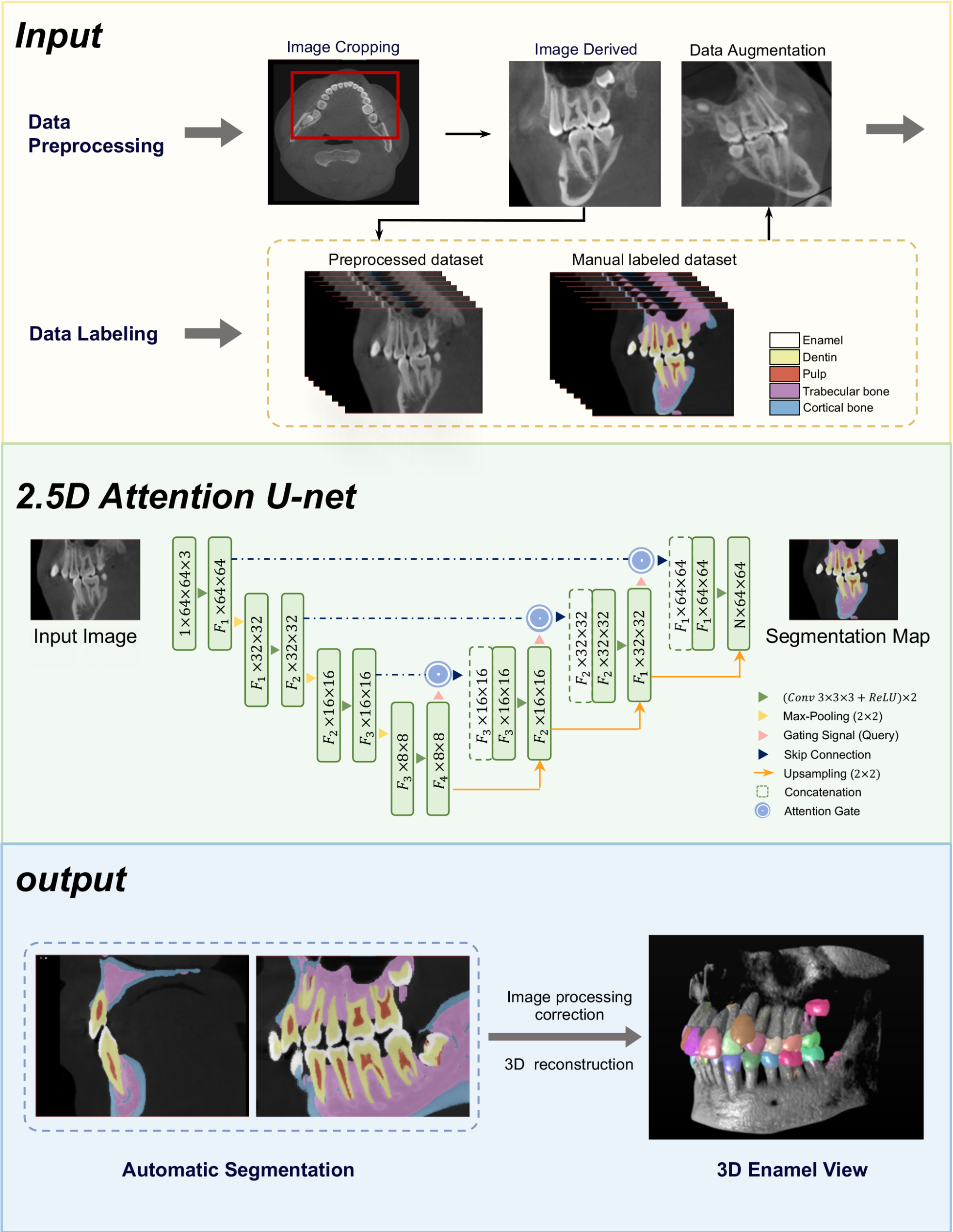
Segmentation model

The segmentation model was based on U-Net because of its proven effectiveness in biomedical image segmentation tasks, especially when dealing with limited data. U-Net’s architecture is particularly well-suited for capturing fine-grained details in images, because of its symmetric encoder-decoder structure.

The encoder path allows the model to capture contextual information through downsampling, whereas the decoder path uses upsampling to restore spatial resolution, ensuring precise localization. Additionally, the skip connections between the corresponding layers in the encoder and decoder allow the model to retain critical high-resolution features, which are essential for accurate segmentation of anatomical structures.

This architecture helps balance the need for both a global context and detailed localization, making U-Net highly effective for medical imaging tasks where precision is paramount. By leveraging U-Net, the model can effectively learn to identify and segment regions of interest from the 1831 axial slices with relatively few training examples, making it a powerful tool for medical image segmentation. The model started by reading the 37 Nii images into 1831 png axial slices. After that, the images were resized to 112 × 112 before the data were split into 1464 slice for training and 367 slice for testing (Fig. 5). The model started training for 80 epochs with a learning rate of 0.00001, the patch size was 16, and the optimizer used was Adam, with a total of 1,940,817 parameters extracted (Fig. 6).

Fig. 5

Pipeline for the U-Net model architecture used for MB2 segmentation

Fig. 6

Diagram of the MB2 segmentation model development steps

Evaluation

The accuracy of the deep learning model (DLM) versus the ground truth (GT) was evaluated via the following 2 methods:

1.

Canal detection accuracy using the classifier DLM:

A dichotomized outcome of “presence of MB2” and “absence of MB2” per MB root of DLM was compared with that of GT, where the GT was determined and agreed upon by 2 maxillofacial radiologists with 8 and 15 years of experience.

The results of the test group were put into a confusion matrix of true positive (TP), false positive (FP) and false negative (FN) parameters, where (TP) is the accurate prediction of the image with MB2, (FP) is the incorrect prediction of the image with MB2 and (FN): is the incorrect prediction of the image without MB2, and (TN) is the correct prediction of the image without MB2.

On the basis of this confusion matrix, the precision, recall (sensitivity) and F1 score were calculated and graded according to the ranking for diagnostic tests by Leonardi Dutra et al. [39], with scores of 80% considered excellent outcomes, scores between 70% and 80% good, scores between 60% and 69% fair, and scores of 60% poor. Roots with 1 canal were used as the control group.

The Accuracy, evaluates the correct predictions generated by the model throughout the complete dataset. The calculation is the ratio of true positives (TPs) and true negatives (TNs) to the total number of samples.

The precision, or positive predictive value, evaluates only true positives among all positive predictions generated by the model. It is determined by the ratio of true positives (TPs) to the total number of true positives and false positives (FPs).

Recall, also referred to as the sensitivity or true positive rate, quantifies the ratio of true positive forecasts to all real positive cases, thereby accounting for missed positives. It is determined by the ratio of true positives (TPs) to the total number of true positives and false negatives (FNs).

F1 score— The F1 score is a statistic that equilibrates precision and recall. It is computed as the harmonic mean of precision and recall.

Accuracy assesses the overall correctness of the model’s predictions, whereas precision and recall concentrate on the quality of positive and negative predictions, respectively. The F1 score offers an appropriate ratio between precision and recall, rendering it a more balanced indicator for assessing classification models. The area under the curve (AUC) of the receiver operating characteristic (ROC) curve was also calculated.

2.

The segmentation accuracy was measured through voxel matching via the Dice similarity coefficient calculated for the root canal label:

The set of pixels labelled as root canals in the segmented image generated by our U-Net-based model was compared with those labelled by the radiologist (GT).

The Dice similarity coefficient, or simply the Dice coefficient, is a statistical tool that measures the similarity between two sets of data. This index has become a common metric in the validation of image segmentation algorithms created with AI.

The equation for this concept is:

\(2\ast\left|\mathrm X\cap\mathrm Y\right|/\left(\left|\mathrm X\right|+\left|\mathrm Y\right|\right)\), where X and Y are two sets:

|X| represents the number of elements in set X (voxels segmented by the DLM), and |Y| represents the number of elements in set Y (voxels segmented by the radiologist (GT)).

∩ is used to represent the intersection of two sets and represents the elements that are common to both sets.