Data collection and preprocessing

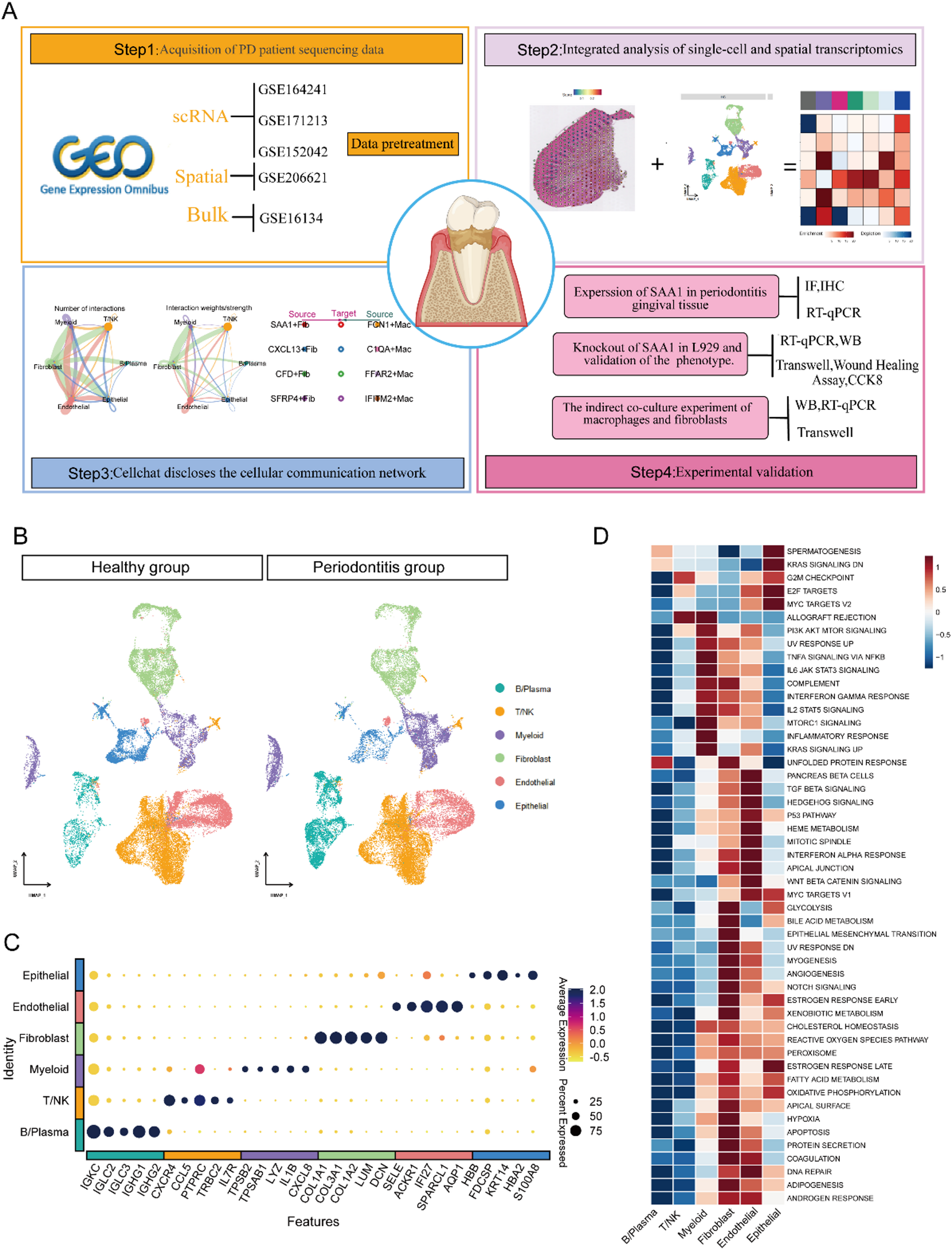
The sequencing data that were used in this study were obtained from the GEO database (http://www.ncbi.nlm.nih.gov/geo). Specifically, our analysis included three scRNA-seq datasets (GSE171213, GSE164241, and GSE152042), one spatial transcriptomics dataset (GSE206621), and one bulk transcriptome dataset (GSE16134). After the data were downloaded, the bulk transcriptome data were log transformed. Comprehensive details about these datasets are summarized in Table 1 in the supplementary materials.

Single-cell data analysis

We imported the scRNA-seq dataset into R (version 4.3.1) and conducted a comprehensive analysis and processing using the Seurat package (v4.4.0) [19]. ScRNA-seq dataset sampling was conducted to ensure optimal integration and to avoid bias toward samples with an excessive number of cells. Three rounds of sampling were conducted on the quality-controlled data, and 1,000 cells were randomly selected from each sample in each round. After duplicate cells were eliminated, the sampled cells from all three rounds were combined, resulting in a total of 65,979 cells from 28 samples (14 healthy control (HC) samples and 14 PD patient samples). This dataset included 32,958 cells from diseased tissues and 33,021 cells from healthy tissues, and these cells were used for subsequent analysis. All the data were normalized using the sctransform method [20]. Harmony (v0.1.0) was used to eliminate batch effects before conducting independent component analysis [21]. UMAP plots are used to display the distribution of cells among different samples or different groups after batch effects have been removed. Cell annotation relies primarily on manual curation, with additional support from SingleR [22]. Marker genes were detected through the “FindAllMarkers” function by applying the Wilcoxon rank sum test. The filtering criteria included a log2-fold change (log2FC) exceeding 0.5, a p value below 0.05, and a “min pct” greater than 0.5. Gene expression levels were then visualized with a UMAP plot using the “FeaturePlot” function.

Gene set variation analysis (GSVA)

GSVA is a gene set scoring method that is commonly used to analyze both bulk samples and single-cell data [23]. To conduct functional enrichment analysis for each cell type, we pre-downloaded the Hallmark gene sets from MSigDB database (http://software.broadinstitute.org/gsea/msigdb) and obtained M1/M2 polarization gene sets from relevant literature [24]. To visually represent the results, heatmaps were constructed using the “pheatmap” package available in R.

Spatial transcriptome data analysis

We utilized the Seurat package in R to import the initial UMI count matrix, associated imaging files, spot locations, and scaling factors. The RNA content variability per spot was normalized using the Sctransform method. Dimensionality was reduced by principal component analysis (PCA), and an elbow plot was generated for each tissue slice to determine the optimal number of principal components. Clustering was performed using the Louvain algorithm with a resolution of 0.3, and the resulting clusters were spatially mapped using the “SpatialDimPlot” function. The expression patterns of individual genes across the slices were visualized with the “SpatialFeaturePlot” function.

Multimodal intersection analysis (MIA)

For the integration of cell type-specific genes that were identified by scRNA-seq and cluster-specific genes that were identified by spatial transcriptomics, we used the MIA method [25], which is based on the hypergeometric test, to evaluate significant enrichment between these two sets of genes. Spatial clusters were characterized as primary regions for specific cell types, marked by the highest enrichment significance when intersected with the respective cell type-specific genes. By combining the signature genes of each cell type from the single-cell data, MIA analysis was conducted to determine the dominant cell types that were present in each spatial region.

CellChat (v1.6.1) analysis

We constructed a cell communication network by applying the “computeCommunProb”, “computeCommunProbPathway”, and “aggregateNet” functions [26]. Circular plots were generated using the “netVisual_circle” function to visualize the communication network. The “netAnalysis_signalingRole_scatter” function was used to create scatter plots showing the strength of the signals that were sent or received by different cell types. To compare the signaling differences among cells in different groups, heatmaps were generated using the “netVisual_heatmap” function. Finally, the “rankNet” function was used to visualize changes in the signal strength of individual components.

NicheNet analysis

NicheNet analysis is used to predict which ligands derived from sending cells regulate the expression of receptors or target genes in receiving cells [27]. We implemented this analysis with the “nichenet_seuratobj_aggregate” function. For differential gene expression analysis, we retained only the genes with a log2FC ≥ 0.4 that were upregulated in the PD samples. All the fibroblast subpopulations were designated as “sending cells”, and the macrophages were designated as “receiving cells”. This approach allowed us to identify a set of predicted fibroblast-derived ligands that may regulate the observed responses in macrophages.

Functional enrichment

We utilized the “FindMarker” function to identify DEGs between SAA1 + Fib and other fibroblast subtypes. These DEGs were subsequently subjected to functional enrichment analysis. GO enrichment and KEGG enrichment analyses were performed with the “clusterProfiler” R package (version 250.3.18) [28]. Additionally, Gene set enrichment analysis (GSEA) was performed with the “Gseavis” package. Pathways with a p value < 0.05 were selected for further investigation. The heatmap in Fig. 4B and its associated functional enrichment results were generated using the “ClusterGVis” tool [29].

Establishment of a PD mouse model via ligation

Periodontitis was induced in 8-week-old male C57BL/6 mice by ligating the bilateral maxillary second molars with a 5–0 suture. Mice that were not subjected to ligation served as controls. The period of model establishment lasted for two weeks. After the experiment, whole blood samples were collected from the mice and centrifuged to isolate the serum, which was subsequently used for ELISA analysis. Next, the mice were humanely euthanized through carbon dioxide-induced-induced asphyxiation, and the mandibles were carefully dissected. The mandibles were sectioned along the midpalatal suture; the left halves of the mandibles were stored at -80 °C for future analysis, and the right halves were fixed overnight in 4% paraformaldehyde (PFA) at 4 °C. After fixation, the samples were thoroughly rinsed with PBS (Servicebio, Wuhan, China) and then subjected to microcomputed tomography (micro-CT).

RNA extraction and RT‒qPCR

Total RNA was extracted from fresh frozen gingival tissues or cultured cells using the MonaZolTM reagent (Monad Biotech, Suzhou, China). The total RNA was subsequently reverse transcribed into cDNA with an RT kit. The RT‒qPCR experiments were conducted using SYBR Green PCR Master Mix. Relative mRNA expression levels were quantified with the 2− ΔΔCT method. To ensure the reliability of the results, all the experiments were repeated three times. Additionally, the GAPDH gene was used as the internal reference gene to normalize the data. The sequences of the primers that were used are listed in Table 2 in the supplementary materials.

Western blot

Cells were lysed with strong protein lysis buffer (Solarbio, Beijing, China), and the proteins were extracted from the cells. The proteins were separated by 10% sodium dodecyl sulfate‒polyacrylamide gel electrophoresis (SDS‒PAGE). After electrophoresis, the proteins were transferred to PVDF membranes (0.45 μm, Millipore, MA, USA) using a rapid transfer buffer (Servicebio, Wuhan, China) supplemented with 20% methanol. After transfer, the membranes were blocked, followed by incubation with primary and secondary antibodies. The signals were then visualized using a chemiluminescent detection system and a gel imaging system (Tanon, Shanghai, China). Information about the antibodies is presented in Table 3 in the supplementary materials.

Histological staining of mouse periodontal tissue sections

After micro-CT reconstruction was complete, the maxillary bone samples were placed in a 10% ethylenediaminetetraacetic acid (EDTA, pH 7.6) solution for 4 to 8 weeks for decalcification. After decalcification, the samples were embedded in paraffin and sectioned. For H&E staining, the paraffin sections were first dewaxed with xylene and rehydrated with a series of gradient ethanol solutions to remove the paraffin and rehydrate the sections. The sections were then stained with hematoxylin followed by eosin according to the manufacturer’s guidelines (Servicebio, Wuhan, China). For IHC staining, the paraffin sections were dewaxed and rehydrated. Specifically, the sections were subjected to antigen retrieval by incubation in sodium citrate buffer at 95 °C for 10 min. This step was followed by incubation with 3% hydrogen peroxide at room temperature for 10 min to inhibit endogenous peroxidase activity. Then, the tissue sections were blocked and incubated with the primary antibody followed by the secondary antibody. Positive signals were detected using DAB or AEC kits (Boster Biological Technology, China). For IF staining, the sections were dewaxed, rehydrated, and subjected to antigen retrieval before they were incubated with primary antibodies overnight at 4 °C followed by Alexa Fluor 488-labeled secondary antibodies. Nuclei were counterstained with DAPI 4080 (UElandy, Suzhou, China). The details about the antibodies that were used are provided in the supplementary materials. Imaging was performed with a 3DHISTECH digital slide scanner (3DHISTECH, Hungary).

SAA1 gene knockout in L929 cells

Suitable target sites were identified using gRNA design software, and multiple sgRNAs were designed for each target site to increase the knockout efficiency, following established principles for optimal target selection. PCR primers were then generated on the basis of the gRNA sequences to amplify the genomic editing sites and facilitate KO genotype analysis. After electroporation, the cells were cultured for 3‒5 days until the cell density was greater than 60%. Samples were collected to assess KO efficiency. Subsequently, a series of procedures were performed, including lysing the cells to form a suspension, preparing PCR, conducting gel electrophoresis, and performing Sanger sequencing. Finally, the sequences of the KO cells were compared with those of the L929 cells to analyze the editing efficiency. The sgRNA sequences and PCR amplification primer sequences are presented in Table 4 in the supplementary materials.

CCK-8 proliferation assay

First, suspended cells were counted and seeded in 96-well plates at a density of 5000 cells per well. The same volume of PBS was added to wells without cells to avoid errors. The CCK-8 reagent (ShareBio, Shanghai China) was diluted 1:100 with serum-free medium and incubated with the cells in the dark at 37 °C for two hours. The absorbance at 450 nm was subsequently measured using a Spectra MAX Absorbance Reader CMAX Plus microplate reader (Molecular Devices, USA) to assess cell proliferation.

Wound healing assay

Cells were seeded in six-well plates and cultured until they formed a monolayer. Then, a 200-µL pipette was used to generate a straight scratch perpendicularly and evenly with moderate force. Loose cells were removed with PBS. Then, the cells were further cultured with serum-free medium, and cell migration was recorded at 0 h, 24 h, 48 h and 72 h.

Transwell migration assay

A cell suspension (100 µL) containing 20 × 104 cells was added to the upper chamber of each Transwell insert (Corning, NY, USA). Next, 500 µL of DMEM (Gibco, MA, USA) supplemented with 10% FBS (ExCell Bio, Suzhou, China) was added to the lower chamber. The plate was incubated at 37 °C in a cell culture incubator for 24 h. Then, the cells that did not migrate from the upper chamber were carefully removed. The bottom of the insert was immersed in 4% paraformaldehyde and incubated for 25 min to fix the cells, which were then stained with 0.1% crystal violet solution for 15 min. Five fields of view were randomly selected under an optical microscope for imaging and recording. ImageJ software was used to count the cells that had migrated.

Preparation of conditioned medium from L929 and L929-KO-SAA1 cells

Cells were seeded in T25 cell culture flasks and cultured in complete medium supplemented with 10% FBS at 37 °C with 5% CO2 until they reached 90% confluence. The complete medium was then discarded, and the cells were washed three times with PBS. Then, serum-free DMEM (Gibco, MA, USA) supplemented with 1% penicillin‒streptomycin (Solarbio, Beijing, China) was added. After 48 h of incubation, the conditioned medium was collected and centrifuged at 1000 × g for 10 min at 4 °C to pellet the cell debris. The supernatant was then filtered through a 0.22-µm filter (Jetbiofil, Guangzhou, China) to remove any remaining cell debris or dead cells.

Cell Immunofluorescence (IF) staining

RAW264.7 cells were cultured in confocal dishes and exposed to conditioned medium for 24 h. For IF staining, the cells were washed three times with PBS, fixed with 4% paraformaldehyde at 4 °C for 15 min, permeabilized with 0.2% Triton X-100 for 10 min, and blocked with 2% BSA for 2 h. Primary antibodies were added, and the samples were incubated overnight at 4 °C. After the samples were washed with PBS, secondary antibodies were added, and the samples were incubated at room temperature for 1 h in the dark. Nuclei were stained with DAPI (UElandy, Suzhou, China) for 1 min. Anti-fade mounting medium was applied before imaging was performed with a confocal laser scanning microscope (OLYMPUS, Japan). Details about the antibodies that were used are provided in the supplementary materials.

Drug screening and molecular Docking

The structure of SAA1 protein was obtained from the PDB (databasehttps://www.rcsb.org/). Based on the resolution of the protein structure, 4IP8 was selected as the representative structure of SAA1 for subsequent molecular docking studies. We screened potential drugs that could target the SAA1 protein through the DGIdb (Drug-Gene Interaction Database) database and obtained the chemical structures of these drugs from the PubChem website (https://pubchem.ncbi.nlm.nih.gov/). Subsequently, molecular docking analysis was performed on the selected drugs and SAA1 protein using AutoDock Tools 1.5.7 software, and the docking results were visualized using PyMOL software. The drug screening results are detailed in Table 5 of the supplementary materials.

Cell viability assay

Cell viability was determined using the CCK-8 method. RAW264.7 cells (at a density of 5 × 10^3/mL) were seeded in 96-well plates, and the initial medium was replaced with complete medium. The cells were then treated with different concentrations of two drugs for 24 h. According to the literature, the concentration gradients of the two drugs were set as follows: Anakinra (0, 100, 200, 400, and 800 ng/mL) [30] and Naproxen sodium (0, 5, 10, 20, and 40 µM) [31]. Subsequently, 10 µL of CCK-8 reagent and 90 µL of fresh medium were added to each well and incubated for 2 h. Finally, the absorbance values were detected at a wavelength of 450 nm. A blank control group without cells was set up, and each group included three parallel samples to ensure data reliability.

Statistical analysis

Statistical analysis was performed with R software, GraphPad Prism 9, and ImageJ. For comparisons between two groups, an unpaired two-tailed t test was used unless otherwise specified. Correlations among variables were assessed with Spearman’s correlation tests. The experimental data are presented as the means ± SDs, and unless otherwise stated, a p value less than 0.05 was considered to indicate a statistically significant difference.