
Remember me
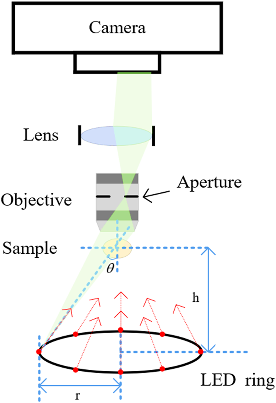
To show the feasibility of the ‘SR-HDS with a built-in denoising function using SR-HDNN’, we perform numerical simulations. Figure 5 illustrates the optical setup assumed in the numerical simulations of SR-HDS and SR-HDNN. The parameters used in the SR-HDS and SR-HDNN simulations are listed in Table 1.
First, we perform the numerical simulation of the writing process of SR-HDS. The summed pattern of the binary SP with a phase difference of \(\pi /2\) and the binary AP with a phase difference of \(\pi\) is used as the WP and is phase-modulated onto a plane wave. The intensity distribution inside the recording medium, I(x, y, z), can be calculated based on diffraction theory and is assumed to be converted into refractive index changes, \(\varDelta n(x,y,z)\), according to the following equation:
$$\begin \varDelta n(x,y,z) = \varDelta n_\textrm \left\}}\right] \right\} . \end$$
(1)
Here, \(\varDelta n_\textrm\) is the maximum refractive index change, t is the recording time, and \(E_}\) is a constant determined by the sensitivity of the recording medium. In addition, a hologram was recorded using a different random WP for the SR-HDNN.
In the reading processes of SR-HDS and/or SR-HDNN, beam propagation must be computed in an inhomogeneous medium, i.e., a hologram. When beam propagation is calculated only once for the hologram, as in the reading process of SR-HDS, we use the fast Fourier transform beam propagation method (FFT-BPM) [17]. However, when beam propagation is calculated iteratively for the same hologram, as in the training process of SR-HDNN, we employ the transmission matrix (TM) method, which establishes the relationship between the complex amplitude distributions on the P-SLM and imager planes [18]. It should be noted that TM can be effective if the system between the input and output planes is optically linear. Once the TM between the P-SLM and imager planes \(M_\textrm\) is obtained, we can immediately calculate the complex amplitude on the imager plane when an arbitrary complex amplitude on the P-SLM plane is given as follows:
$$\begin }_\textrm = M_\textrm }_\textrm \end$$
(2)
where \(}_\textrm\) and \(}_\textrm\) is 1D-expression of the complex amplitude distribution on the P-SLM and imager planes, respectively.
To measure the TM of the optically linear system, an \(N \times N\) Hadamard matrix \(M_\textrm\) is first prepared. Each column of \(M_\textrm\) is extracted, converted into a 2D distribution, and modulated onto a beam on the P-SLM plane. Here, ‘1’ and ‘-1’ is interpreted as ‘0’ and ‘\(\pi\)’ phase modulation, respectively. Next, the propagation of the beam through the system is calculated and the complex amplitude distribution on the output plane is measured. Subsequently, we use FFT-BPM for the beam propagation through the system. This procedure is repeated for all the columns of \(M_\textrm\), and the resulting output complex amplitude distributions are recorded as matrix \(M_\textrm\). Consequently, we can obtain the relationship between \(M_\textrm\) and \(M_\textrm\):
$$\begin M_\textrm M_\textrm = M_\textrm. \end$$
(3)
Therefore, TM can be obtained immediately as follows:
$$\begin M_\textrm = M_\textrm M_\textrm^\textrm. \end$$
(4)
where \(\textrm\) denotes the transpose matrix.
To evaluate the denoising performance, we used the SNR defined by the following equation:
$$\begin \textrm = \frac_\textrm - \bar_\textrm}+\sigma ^2_\textrm}}. \end$$
(5)
Here, \(\bar_\textrm\) and \(\bar_\textrm\) are the mean values of the reconstruction intensities corresponding to the ON and OFF pixels, respectively. Similarly, \(\sigma _\textrm\) and \(\sigma _\textrm\) are the standard deviations of the reconstruction intensities corresponding to the ON and OFF pixels, respectively. A higher SNR value indicates better quality of the reconstructed datapages.
In this study, we conduct three simulations using the ‘SR-HDS with a built-in denoising function based on SR-HDNN’. First, we evaluate the feasibility of denoising using SR-HDNN by following the image flow shown in Fig. 4. To train SR-HDNN, we generate a dataset of recorded and reconstructed SP pairs using SR-HDS simulations. Second, we conduct the same evaluation as in the first simulation but with a different dataset generation approach. Instead of directly obtaining the dataset from the SR-HDS simulations, we performed a significantly smaller number of simulations to analyze the statistical properties of noise. Using these properties, we generated artificial SPs that significantly reduced the time required for dataset creation. Finally, we applied a second simulation to evaluate the amount of noise that could be removed using the proposed method.
Fig. 5
Numerical simulation model
Table 1 Simulation parameters4.1 Denoising demonstration with reconstructed images acquired by SR-HDS simulationWe evaluate the feasibility of denoising using SR-HDNN by following the image flow shown in Fig. 4. First, we perform simulations of the writing and reading processes for 1,400 SPs based on SR-HDS. Next, SR-HDNN is trained using 1,400 pairs of original and reconstructed SPs. The training conditions are presented in Table 2. Finally, we test the denoising performance of SR-HDNN using 100 reconstructed SPs that were not used during training.
Figure 6 shows the reconstructed SPs before and after denoising, along with the mean SNR values and standard errors. After denoising, the reconstructed datapages exhibit improved SNR values, demonstrating that SR-HDNN effectively enhances the quality of the reconstructed SPs. It appears that SR-HDNN was trained to reduce the variance in the difference between the ON and OFF intensities of SPs rather than to increase the difference. In other words, it improves the SNR by reducing the denominator in Eq. 5. This characteristic is likely to vary depending on the training conditions, such as the loss function, dataset, and other factors.
Table 2 Training conditions for SR-HDNNFig. 6
a Original and denoised datapages. b SNR of original and denoised datapages
4.2 Denoising demonstration with artificial reconstructed imagesIn the simulation described in the previous section, the dataset used for training was obtained through SR-HDS. However, this method requires a long time to generate a dataset. Additionally, when applying the proposed method to a practical HDS system, repeated recordings and reconstructions are necessary to create a dataset. Therefore, we tested an alternative approach to artificially generate reconstructed SPs for the dataset based on the noise characteristics of several reconstructed SPs obtained through multiple SR-HDS simulations.
First, we generated artificial datapages that replicated the amplitude noise characteristics of the reconstructed datapages in the SR-HDS. Specifically, we analyzed the amplitude variances of the noise superimposed on the reconstructed datapages obtained in Sect. 4.1. Figure 7a shows an example of 1400 reconstructed datapages obtained through the SR-HDS simulations, along with their corresponding histograms. The simulation results show that Gaussian noise is superimposed on the reconstructed datapages. This noise arises from variations in the intensity of inter-pixel interactions during the reading process, as the distance and number of interacting pixels vary depending on the position of each pixel. In practice, random noise sources such as scattering and electrical noise are also present in addition to Gaussian noise. However, since Gaussian noise is expected to be the most dominant, only Gaussian noise is considered in the following simulations.
Based on the extracted amplitude variances, we generated artificial datapages by adding noise to randomly generated distributions using image processing techniques. Figure 7b shows an example of 1,400 artificially created datapages and their corresponding histograms. We qualitatively confirmed that the artificially generated datapages effectively replicated the intensity distribution of the reconstructed datapages obtained from the SR-HDS simulation.
Subsequently, we trained SR-HDNN using the artificially generated datapages and applied it to the denoising task. The optical system and training conditions were the same as those listed in Tables 1 and 2. The evaluation results of the quality improvement through denoising are presented in Fig. 8. Figure 8a shows datapage images before and after denoising, whereas Figs. 8b illustrates the change in SNR, with error bars indicating the standard error. The denoised reconstructed datapages exhibit improved SNR values, demonstrating the effectiveness of using artificially generated datapages for train the denoising process.
Fig. 7
a Reconstructed datapage and its histogram. b Artificially generated datapage and its histogram
Fig. 8
a Original and denoised datapages when artificially generated datapages are used as dataset. b SNR of original and denoised datapages when artificially generated datapages are used as dataset
4.3 Denoising capabilityIn this section, we investigate the maximum level of Gaussian noise that can be effectively denoised using SR-HDNN. To this end, we generated artificially noisy datapages by adding Gaussian noise with specific standard deviations and evaluated the quality improvement ratio after denoising. The artificially generated datapages were used for both training and denoising. Specifically, we varied the standard deviation of the noise from 0.09 to 0.20 in increments of 0.01 and performed denoising using SR-HDNN. The optical system and the training conditions were the same as those listed in Tables 1 and 2. Figure 9 shows the relationship between the standard deviation of noise in the artificially generated datapages and the SNR after denoising. As the standard deviation of the noise increased, the SNR decreased. When the standard deviation exceeded 0.18, the SNR improvement ratio dropped below 1.0. These results indicate that the denoising capability of the SR-HDNN has an upper limit, and under the given simulation conditions, it is effective for noise with standard deviations up to 0.17.
Fig. 9 4.4 Discussions
We numerically demonstrated the ‘SR-HDS with a built-in denoising function based on SR-HDNN’ and confirmed that SR-HDNN is effective in denoising reconstructed datapages in SR-HDS. Furthermore, we verified that both numerically reconstructed datapages and artificially generated datapages can serve as training data. Compared to the reconstructed datapages obtained through numerical simulations of SR-HDS, artificially generated datapages can be created at a lower computational cost, thereby improving the efficiency of the denoising system when used as training data. Additionally, our results indicate that the denoising capability of SR-HDNN has an upper limit. Consequently, we have demonstrated the feasibility of the ‘SR-HDS with a built-in denoising function based on SR-HDNN’.
There are several potential approaches to improving denoising quality. In this simulation, while the SNR improved, the training process not only reduced the intensity variance of the ON and OFF pixels but also decreased the mean intensity difference between them. It is believed that finding a more appropriate loss function and adjusting the training conditions could further. Additionally, SR-HDNN could control the inter-pixel interaction of the RP, which is phase-modulated onto the beam by the NP. In other words, the hologram recorded for SR-HDNN can be controlled by the NP. Preparing a separate hologram for SR-HDNN and studying the optimal recording strategy for denoising would also be beneficial. Furthermore, an experimental verification of the proposed method is required. However, some challenges must be overcome. For instance, it has been pointed out that even slight changes in the optical system during the training and denoising processes can hinder the training process when using the TM of the system [19]. In other words, TM-based training cannot account for temporal variations in noise, making it difficult to experimentally demonstrate the method using current training approaches that do not maintain consistent TMs during training and denoising. Although the conclusions regarding the feasibility of the proposed method presented in this paper remain unchanged, we plan to conduct experimental verification in future by considering the adoption of training strategies developed for other physical neural networks, which improve the robustness of TPs by incorporating experimental noise into the training process. In particular, we consider algorithms such as physics-aware training (PAT) [20, 21], which combines forward propagation through a physical device with backpropagation using the TM, and direct feedback alignment (DFA) [22,23,24,25], which enables direct training on a physical device without requiring the TM. We also explore strategies based on these algorithms, such as the adaptive training method [26], to address implementation errors in numerically designed models by training them directly on physical systems.
Comments (0)