
Remember me
For the study at hand, we generate and utilize three distinct datasets: RadPHI-train as our training dataset and two evaluation datasets, RadPHI-test and MIDI. RadPHI-train and RadPHI-test are created by overlaying synthetically generated imprints on curated medical images across various modalities. MIDI is created by overlaying information stored in DICOM tags, which may contain PHI, utilizing an industry standard DICOM viewer. The RadPHI-train is used to develop our text detection model, while the RadPHI-test is employed to evaluate different configurations of the PHI detection pipeline. Additionally, the MIDI dataset is reserved as a hold-out test set to assess the optimal configuration identified through the RadPHI-test evaluation. In the upcoming sections, we will elaborate on the generation process for each of these datasets.
PHI DefinitionFor data simulation and evaluation, we define a list of PHI and non-PHI items based on the HIPAA guidelines [1] as detailed in Table 1. The six PHI categories include date, general identifier, patient name, address, phone number, and email. We group all identification numbers into a group of identifiers, including patient ID, insurance number, social security number, and any number or series that can be used to identify an individual. The ten non-PHI categories include age < 90, gender, height, weight, examination type, hospital, marker, scanner, diagnosis, and imaging personnel.
Table 1 Imprint categories and examples. There are 16 categories, six of which are classified as PHIPreprocessing of Public DatasetsFor the generation of RadPHI-train and RadPHI-test datasets, we curate radiological images from well-known publicly available datasets. Each of them was preprocessed before we added simulated imprints. In the following, we briefly describe each dataset and the applied preprocessing.
Total Segmentator v2[21] This dataset was originally published and used in a segmentation model for major anatomic structures in CT images. We use the second version, which includes 1228 CT examinations across 21 scanners. Each volume is resampled to isotropic spacing of 0.45 mm across all three planes. Afterwards, four 2D axial slices are uniformly sampled per volume, which makes a total of 4896 2D images. The images are min-max normalized to 8-bit format with the minimum value being random between the 0th and 10th percentile of the image intensities.
BS-80K[22] This dataset includes 82,544 radionuclide bone scan images of 13 body regions designed for classification and object detection tasks. Experts de-identified and annotated the images for classification and object detection tasks. For our experiments, we select subsets of whole-body images in anterior and posterior views. Due to the small size of whole-body images, we create image collages of three to five randomly repeated images. This approach mimics a bone scan viewer, where multiple views of a subject are displayed side by side for comparison. To enhance the diversity of bone scan variants, backgrounds are randomly flipped. The processed images are then saved in 8-bit format.
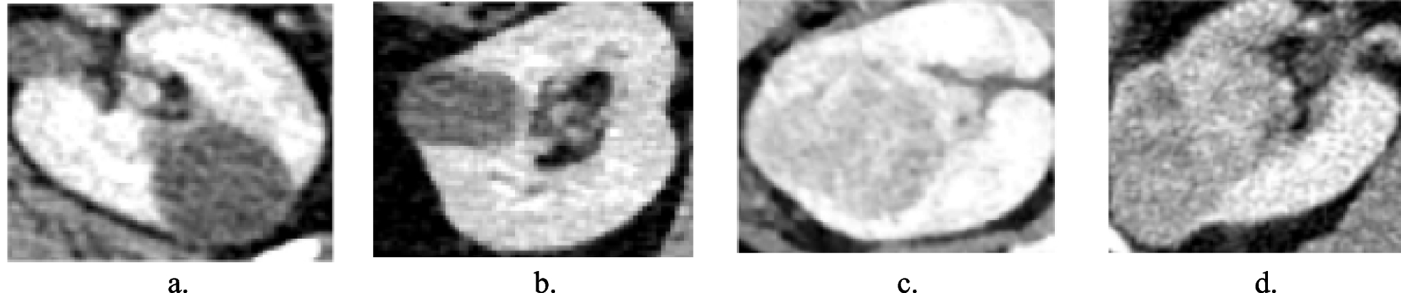
Fig. 3
Imprint simulation pipeline and examples. Given the input PHI ratio for each dataset, each image can have no imprints, non-PHI imprints, or at least one imprint that contains PHI (left). The maximum of imprints per image is eight. Examples of images with imprints across four modalities (right): (a) whole-body CT, (b) whole-body bone scan, (c) chest X-ray, (d) brain MRI
ChestX-ray8[23] This dataset contains 108,948 frontal X-ray images with nine disease labels parsed from radiological reports. Many images contain physical markers indicating left and right direction. To avoid confusion with added text imprints, we use an object detection model to identify these markers and apply center cropping to remove them. After cropping, the images are saved in 8-bit format.
BRATS[24] This dataset is part of the Medical Segmentation Decathlon and includes 750 brain MRI images from four sequences: native T1, post-contrast T1, T2-weighted, and T2-FLAIR. All images are resampled to isotropic spacing of 1 mm. For each subject, a random sequence is selected, and four 2D axial slices are uniformly sampled. The images are then min-max normalized to 8-bit format, following a similar approach to the Total Segmentator v2 dataset.
RadPHI-trainThe main use of the RadPHI-train dataset is to enhance the robustness of the text localization module (see Section 3) against diverse radiological image backgrounds, varying numbers of imprints, and different imprint representations. This dataset is generated based on images from TotalSegmentator, BS-80K, and ChestX-ray8, applying the preprocessing techniques outlined in Section 2.2. Additionally, we simulate imprints on synthetic backgrounds, incorporating plain grayscale colors along with or without multiple boxes in various shades. The text localization module is trained to manage diverse representations of the imprint rather than focusing on its text content. To achieve this, we continuously simulate the imprints using different fonts, sizes, colors, and locations. These imprints may overlap with each other or with anatomical structures. Although such overlaps are not typically seen in real-world data, we intentionally include them as challenging cases for the model to adapt to. A sample from this dataset is shown in Fig. 11 (left) in the Supplementary Material. In total, we generate 6000 images, which are then divided into training and validation sets using an 80–20% split.
Fig. 4
Distribution of PHI categories in the RadPHI-test and MIDI datasets. In the RadPHI-test dataset, each image can have a maximum of one imprint per category. In contrast, the MIDI dataset allows for multiple imprints of the same category in each image. We compute the distribution of PHI categories in the MIDI dataset at the image level, meaning that regardless of the number of imprints for a particular category, it is counted as one
RadPHI-testThe RadPHI-test is designed to evaluate various configurations of our PHI detection pipelines. To achieve this, we create a dataset that simulates real-world image imprints as closely as possible. The imprint simulation process is illustrated in Fig. 3 (left). Based on the input ratio of PHI imprints for the simulated dataset, we determine for each image whether (1) no imprints are added, (2) only non-PHI imprints are added, or (3) at least one imprint includes PHI. Each image can contain a maximum of eight imprints. For each imprint category, as listed in Table 1, we generate imprints in the format <accompanying text><separator><main text>. The accompanying texts consist of signal words that indicate the category of the main text. The separator can be a comma , or a space. For example, in the text Patient Name: John Doe, Patient Name serves as the accompanying text, : is the separator, and John Doe is the main text. In some cases, we randomly omit the accompanying text, such as with identifiers where imprints may consist solely of a sequence of numbers. This omission tests the language model’s ability to infer the underlying imprint category robustly. After adding the imprints, a corresponding label file is generated. This label file contains the coordinates of each imprint in the image, along with its associated PHI class and sub-class. These labels are used for subsequent evaluation. The final dataset used to evaluate the PHI pipeline consists of 1000 images distributed equally across four modalities. Of these, 850 images (\(85\%\)) contain at least one PHI imprint. The distribution of the 16 imprint categories and the number of imprints per image are depicted in Figs. 4 and 5.
Fig. 5
Distribution of PHI and non-PHI imprints in RadPHI-test and MIDI datasets. In RadPHI-test, the number of imprints is limited to eight. In contrast, MIDI has significantly more imprints, correlating to the various DICOM tags and modality-specific imprints randomly displayed on the viewer
Fig. 6
An example of an image from the MIDI dataset featuring PHI overlays. The same PHI element, such as dates, may appear in various contexts, including patient comments and image series. Besides overlays added by the DICOM viewer (left and right), there are burn-ins by the organizer of the MIDI-B challenge (middle)
MIDIThe MIDI dataset is designed to be a challenging hold-out dataset with realistic imprint visualization and placement via a modern DICOM viewer rendering. The image data is curated from the validation and test set of the 2024 Medical Image De-Identification Benchmark (MIDI-B) challenge [25] and is available on The Cancer Imaging Archive [34]. This dataset originally consists of 605 studies across multiple modalities, each containing synthetic PHI content embedded at both the DICOM header and pixel level. We utilize a DICOM viewer, specifically MD.ai [26], to overlay the DICOM tags onto the images. We randomly sample DICOM tags to ensure that the generated imprints represent all possible PHI categories, similar to the RadPHI-test dataset. After applying the overlays, we export the images from the viewer. The resulting images may include not only the DICOM tag overlays but also burn-ins by the challenge organizers. The final version of the dataset comprises 550 images categorized into five PHI types. The category Email is omitted because emails are neither burned in nor inserted into the header of the original dataset. In contrast to the RadPHI-test dataset, each image can have multiple imprints of the same PHI category. For instance, as illustrated in Fig. 6, dates may appear in various contexts, such as the study date, image series, or even the patient comments. We performed instance-level annotation of the images by generating coordinates for PHI instances along with their corresponding categories. This annotation process was carried out and validated by two independent annotators to ensure accuracy and reliability. Figure 4 displays the distribution of PHI categories at the image level. Dates and patient names are among the most frequently occurring PHI elements in the dataset. While we intentionally limit the number of imprints to eight in RadPHI-test, the number of imprints in MIDI can be up to 89, with the majority between 10 and 30 per image (Fig. 5).
Comments (0)