Experimental data collectionParticipants and instrumentation

Seventeen healthy voluntary participants (8 males, 9 females; age: 32 ± 13 years; height: 175 ± 18 cm; body mass: 72 ± 20 kg) were recruited for this study. Inclusion criteria were: (i) self-reported good general health, (ii) no history of upper limb musculoskeletal injuries or neuromuscular disorders, and (iii) ability to perform maximal voluntary elbow flexions without pain or discomfort. Exclusion criteria included: (i) current upper limb pain or injury, (ii) recent engagement in upper-body strength training within 48 h before testing, and (iii) consumption of caffeine, alcohol, or participation in vigorous physical activity within the same 48-h period. Before participating, each individual provided written informed consent, which had been approved by the Research Ethics Committee of La Coruña-Ferrol. The subjects’ arm, forearm, and hand were measured to later scale the subject-specific models.

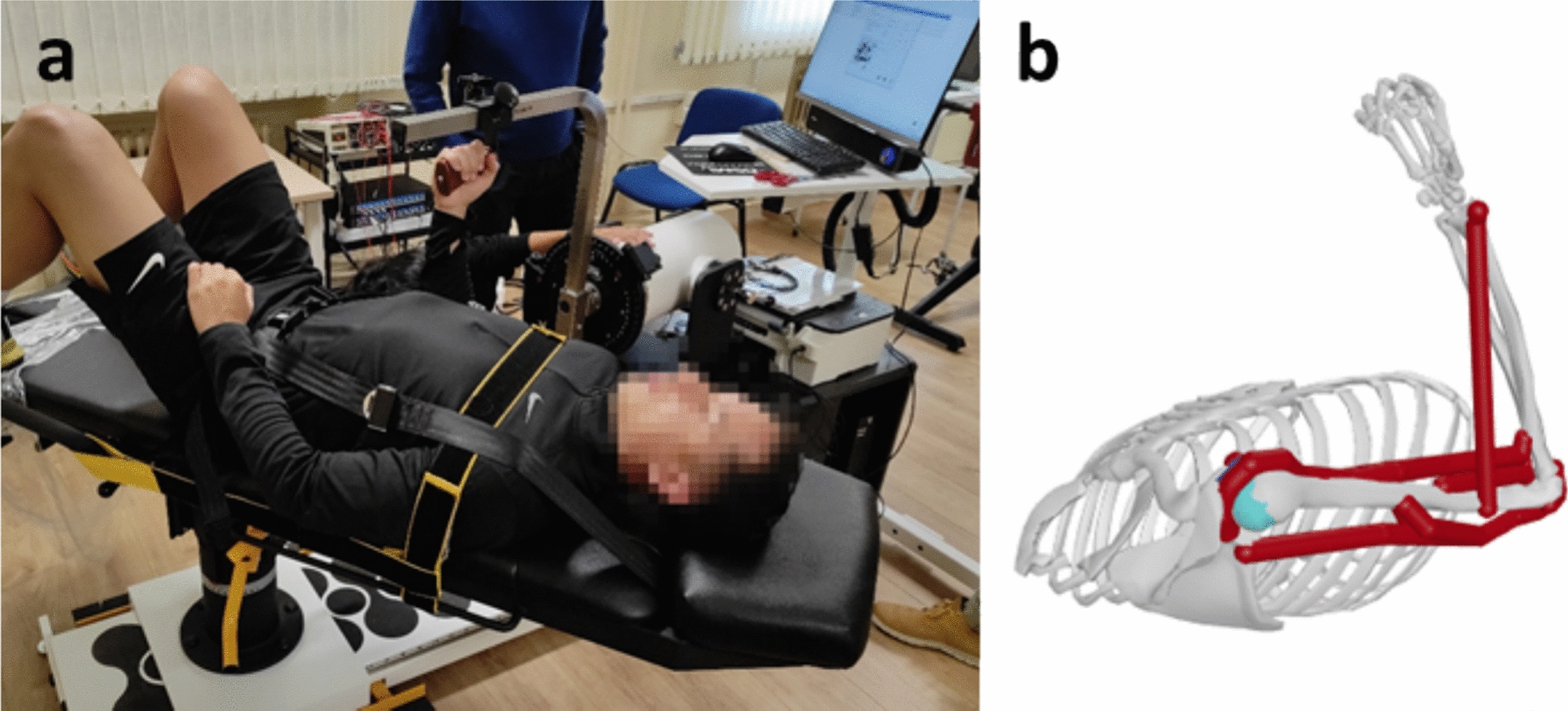
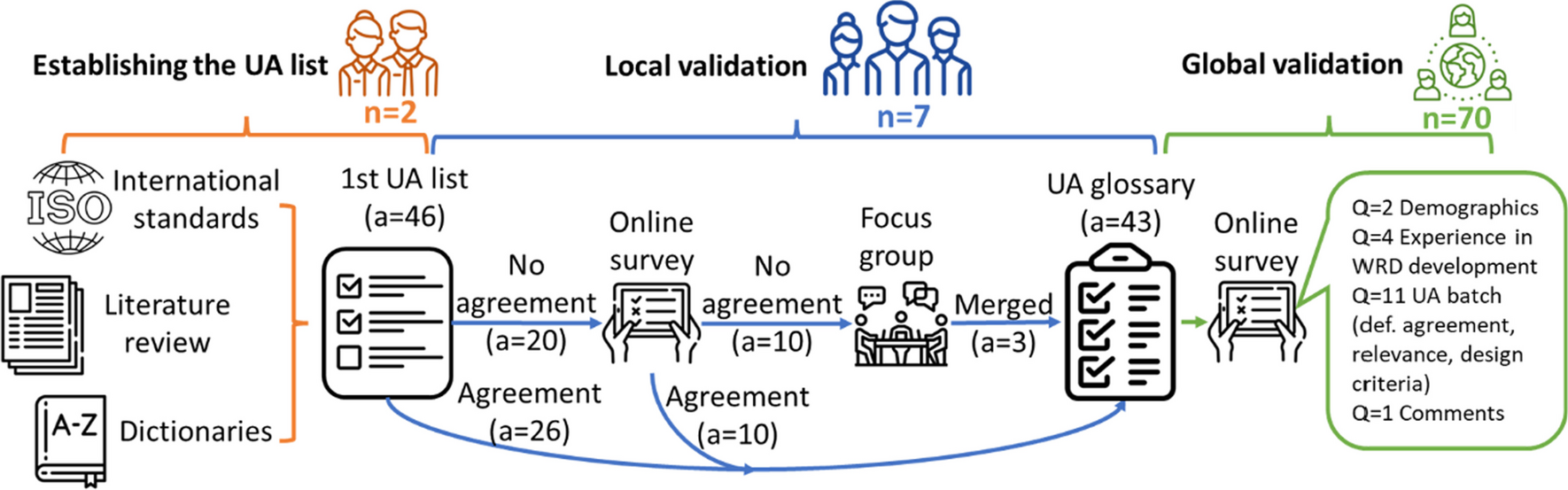
The HUMAC Norm isokinetic dynamometer (CSMi, Stoughton, MA, sampled at 100 Hz) was used to record joint angle and torque generated by the participants. Each subject was positioned in a lying posture and securely restrained to ensure that only the right elbow could move, as shown in Fig. 1a.

Fig. 1

a Isokinetic dynamometer; b 7-muscle arm model

Experimental procedures

Participants followed both an isometric and an isokinetic exercise protocol on the same day. At the start of the session, they completed a 5-min warm-up using a resistance band to reduce the risk of injury. To ensure familiarity with the evaluations and instructions, a simulated recording was made beforehand for each task. Task-specific guidelines, including the number of repetitions, pace, and rest periods, were provided both verbally and visually on a screen positioned next to the subject. During all exercises, participants were instructed to exert maximum voluntary contraction (MVC) and received verbal encouragement throughout [37].

The isometric exercise protocol (hereafter referred to as ISOM6) began with two MVCs, each held for 5 s, at six different elbow flexion angles (15°, 30°, 45°, 60°, 75°, and 90°) in a randomized order. The higher peak force of the two MVCs was retained, and the difference between the two MVCs was checked to ensure it did not exceed 10%. A 45-s rest period was given between the two MVCs of each angle, and a 2-min rest between the MVCs of different angles to minimize the effects of muscle fatigue. After a 5-min rest, participants performed a 30-s sustained MVC at 45°, followed by two additional 5-s MVCs, with rest intervals of 15 s and 60 s, respectively, to measure recovery. Since this exercise induced metabolic inhibition, participants were given a minimum of 30 min of rest before proceeding with the isokinetic protocol.

The isokinetic exercise protocol began with two MVCs during concentric elbow flexion from 15° to 90° at a speed of 15°/s (5 s duration). This ensured participants exerted maximum force throughout the entire range of motion, without fatiguing and allowing the dynamometer to accurately measure it. Additionally, the initial 10° of both eccentric and concentric contractions were excluded from calibration to avoid the effects of the muscle’s response time to excitation. Next, subjects performed two MVCs during eccentric elbow flexion, where they resisted the machine as it extended their arm from 90° to 15° at the same speed and duration. The speed of this exercise not only aimed to achieve maximum effort like the previous one, but also served to reduce the risk of injury, as the machine exerts significant torque. For both exercises, a 45-s rest period was given between each MVC, with a 2-min rest between the two sets. The four sets of measurements (two concentric and two eccentric) were later used in the simulation, and the protocol is referred to as DYN. Finally, after a 5-min rest, participants performed a dynamic, short-duration, high-intensity exercise (DYN-FAT). This involved sustaining an MVC during 4 concentric (15°–90°) and eccentric (90°–15°) elbow flexions (40-s total duration), followed by two additional 5-s isometric MVCs at 45°, with 15-s (DYN-FAT-R1) and 60-s (DYN-FAT-R2) rest intervals, respectively, to measure recovery.

ModelsMusculoskeletal model

The musculoskeletal model used in this study consisted of four segments—trunk, upper arm, forearm, and hand—with a single degree of freedom, allowing only elbow flexion and extension (Fig. 1b). All other joints were fixed and set to match the subject’s posture during the experimental setup (Fig. 1a, b). It incorporated seven muscles: the long, medial, and lateral heads of the triceps; the long and short heads of the biceps; the brachioradialis; and the brachialis. Adapted from [38], the bone geometries were scaled to match each subject’s anthropometric measurements. By combining this model with the recorded joint angles from the isokinetic dynamometer, MTU lengths and moment arms were determined for the exercises.

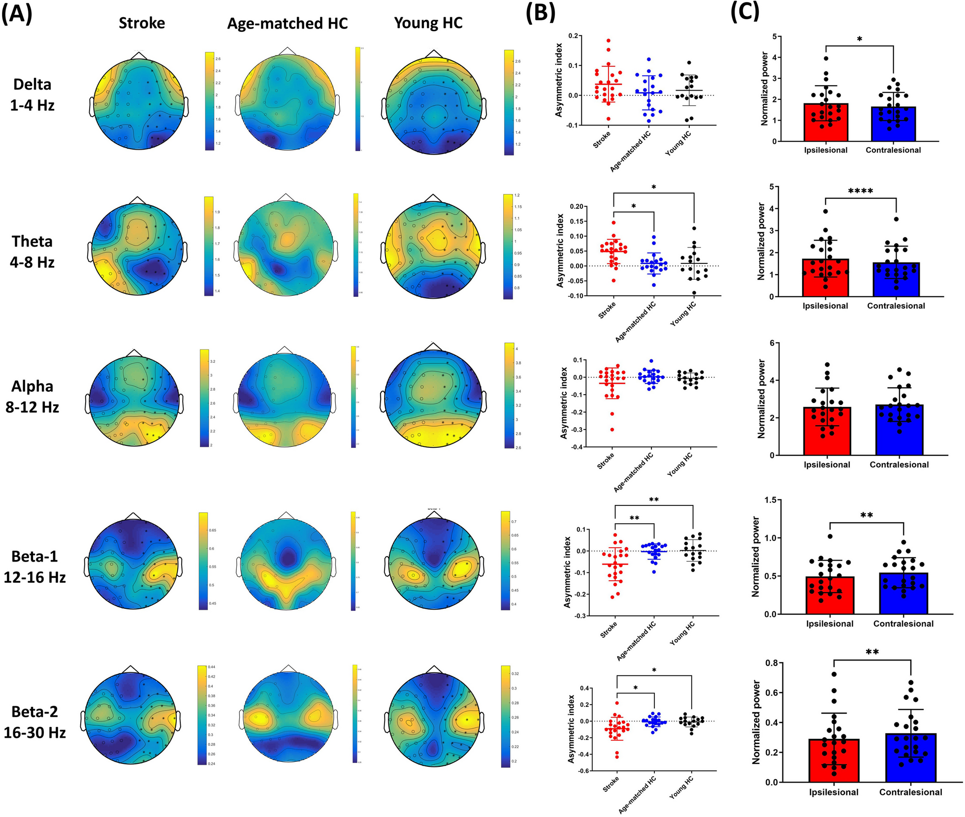
Musculotendon models

Two types of musculotendon models were used to estimate MTU force. The first was a Hill-type musculotendon model [32] (Fig. 2), which accounts for physiological force constraints. The force generated by a MTU depends on its maximum isometric force, as well as its force–length-velocity properties, and is provided by:

$$F^ = \left( ^ + F_^ } \right)\cos \alpha ;$$

(1)

Fig. 2

Hill-type musculotendon model. The MTU fibers are modeled as an active contractile element (CE) in parallel with a passive elastic component (PE). These elements are in series with a nonlinear elastic tendon (SE). The pennation angle α denotes the angle between the MTU fibers and the tendon. Superscripts MT, M, and T indicate musculotendon, MTU fiber, and tendon, respectively [28]

In this equation, \(F_^\) and \(F_^\) represent the forces generated by the contractile element (CE) and the passive element (PE), respectively, while \(\alpha\) corresponds to the pennation angle. The active force produced by the CE is influenced by MTU fiber length, contraction velocity, and activation level, and is defined as:

$$F_^ = F_^ \times a \times f_ \left( } \right) \times f_ \left( } \right);$$

(2)

where \(l^\) is the MTU fiber length, \(v^\) is its velocity, and \(f_\) and \(f_\) are dimensionless force–length and force–velocity relationships, respectively. Since the authors aim to integrate the findings of this study into their real-time human motion capture and musculoskeletal analysis system [39], the tendon is assumed to be rigid, meaning that its length remains constant. This assumption reduces the numerical stiffness of the Hill-muscle equations [40, 41], and significantly decreases the computational time required for simulations while preserving the key physiological considerations [42]. As a result, MTU fiber length and velocity are determined solely by musculoskeletal geometry and segment motion, independently of the musculotendon force. Moreover, to further achieve this objective, the muscle’s time response to excitation is ignored, assuming that activation follows excitation instantaneously, where activation a equals excitation u. This simplification is justified by the fact that the time delays involved are minimal compared to the duration of the exercises analyzed—muscles had sufficient time to reach maximum activation—and, in the context of fatigue, the effect of activation delays would be largely compensated by the corresponding deactivation delays. In Fig. 2, \(l^\) stands for the musculotendon length and \(v^\) is the musculotendon velocity.

The force of the parallel passive element, \(F_^\), which opposes MTU stretch, can be formulated as:

$$F_^ = F_^ \times f_ \left( } \right);$$

(3)

where \(f_\) is a dimensionless force–length relationship, which has non-zero values when the MTU length is greater than the optimal MTU fiber length (\(l_^\)).

In this study, subjects were instructed to produce their MVC to avoid the load-sharing problem. Without this approach, it would be impossible to calibrate maximum forces and determine whether variations in experimental torques were caused by muscle fatigue or by voluntary reductions in muscular activity. Therefore, the activation of the elbow flexors was assumed to be 1 (maximum), while the activation of the elbow extensors was set to 0 (minimum, with no co-contractions). Consequently, the instantaneous allowed forces in flexor and extensor muscles, \(F_}^\) and \(F_}^\), were calculated using \(a\) = 1 (maximal active contraction) and \(a\) = 0 (no active contraction), respectively. In this way, by combining Eqs. (1–3), the resulting flexor and extensor single MTU forces, \(F_^\) and \(F_^\), in muscle i, are represented by Eqs. (4) and (5), respectively.

$$F^ = \left( \left( } \right) \times f_ \left( } \right) + f_ \left( } \right)} \right)F_^ \times \cos \alpha ;$$

(4)

$$F^ = f_ \left( } \right) \times F_^ \times \cos \alpha ;$$

(5)

The second model was a simplified static model that does not account for musculotendon actuator dynamics. In this model, the musculotendon force (\(F_^\)) is directly related to MTU activation (\(a\)) and maximum isometric force (\(F_^\)):

$$F_^ = a \times F_^ ;$$

(6)

Consequently, using the static model, the force of flexor MTUs is \(F_^ = F_^\) and the force of extensor MTUs is \(F_^ = 0\) during elbow flexion MVC. Due to its simplicity, this model only requires the calibration of the maximum isometric force and offers good computational efficiency. Moreover, it has not shown significant differences compared to more physiologically realistic models during gait [42].

Muscle fatigue model

Muscle fatigue is a complex phenomenon influenced by both physiological and psychological factors, leading to a reduced ability to generate maximal force or power during contractile activity. It can occur at different levels of the motor pathway, and is generally classified into central and peripheral fatigue. Central fatigue refers to a decline in the central nervous system’s ability to transmit neural signals to the muscles, resulting in diminished muscle performance [43]. In contrast, peripheral fatigue occurs at the neuromuscular junction and within the muscle itself, involving mechanical and cellular alterations [44]. The recovery of voluntary force-generating capacity after exercise varies, with brief high-intensity exercise typically allowing for rapid recovery, and long-duration exercise often resulting in only partial recovery [45]. To simulate the task-related muscle fatigue for dynamic movements, this work implements a compartment model to characterize muscle activation (Ma), fatigue (Mf), and recovery (Mr) across any target load (TL) [46]. Specifically, the authors adopted the innovative four-compartment (4CC) model which differentiates between short-term fatigue (\(M_^\), associated with metabolic inhibition) and long-term fatigue (\(M_^\), simulating central fatigue and potential microtraumas) [29]. The portion of each subject’s maximum force available at the joint level reflects the proportion of non-fatigued MTUs (RC), accounting for both short-term and long-term fatigue. It is expressed as:

$$RC = \left( ^ + M_^ } \right)} \right)/100;$$

(7)

Consequently, accounting for fatigue, the maximum force that the flexor MTUs can generate within the static musculotendon model during MVC (\(a\) = 1) can be expressed as:

$$F_^ = F_^ \times RC;$$

(8)

Then, considering that peripheral and central fatigue primarily affect the contractile component of MTU force production, only \(F_^\) (2) will be influenced by the muscle’s fatigue level. Consequently, the reduction in maximum MTU force permitted in the elbow flexor MTU during MVC within the physiological model can be formulated as follows:

$$F^ = \left( \left( } \right) \times f_ \left( } \right) \times RC + f_ \left( } \right)} \right) \times F_^ \times \cos \alpha ;$$

(9)

Torque calculation

The net elbow joint torque at each moment during the tasks can be expressed, in a general form, as:

where \(}^\) is the vector of the individual MTU forces, \(}\) is the Jacobian whose transpose projects the MTU forces into the joint drive torque space (i.e., represents the moment arms), and \(Q\) is the resulting elbow joint torque.

The experimental joint torque (\(Q_\)) was directly recorded using the isokinetic dynamometer.

Subject-specific scaling or calibration of musculotendon parameters

Since mechanical and physiological factors influence MTU forces during joint angle variations, three different datasets were compared for calibration:

A single isometric MVC at 60° (ISOM1).

Six static experimental measurements of isometric MVCs (ISOM6).

An isokinetic calibration task, including both concentric and eccentric contractions (DYN).

The following musculotendon parameters have been calibrated or optimized in this study:

Maximum isometric force

Since the relative target load of a task depends on the force exerted by the subject, the maximum isometric force (\(F_^\)) is one of the most critical subject-specific parameters to calibrate. In most studies, this parameter is adjusted to ensure that MTUs can generate the required joint torques [35, 47], sometimes by artificially increasing \(F_^\) or incorporating residual actuators into the model. According to the OpenSim documentation, these residual actuators are referred to as “the hand of God,” as they compensate for discrepancies between model, recorded movements and MTU forces that fail to produce sufficient accelerations [48]. In fatigue studies, overestimating \(F_^\) leads to an underestimation of fatigue, while underestimating it exaggerates fatigue effects. Therefore, correct calibration of \(F_^\) is essential to accurately approximate the subject’s force and fatigue limits, ensuring that MTU forces can generate the required joint torques without being underactivated.

Since the variation of MTU moment arms across joint angles differs among muscles, optimizing individual MTU forces provides greater flexibility for the model to align with experimental measurements without altering the moment arms. Modifying moment arms would require adjusting the coordinates of MTU and tendon attachment sites, leading to significant structural changes and collateral consequences.

Length parameters

The scaled tendon slack length (\(l_^\)) and the scaled optimal MTU fiber length (\(l_^\)), which influence the dimensionless force–length function, were obtained from OpenSim [38] after adjusting the model to match anthropometric measurements. Nevertheless, to determine the best subject-specific calibration strategy, a second scaling was also applied to \(l_^\) by including this parameter in the list of variables to optimize in ISOM6 and DYN.

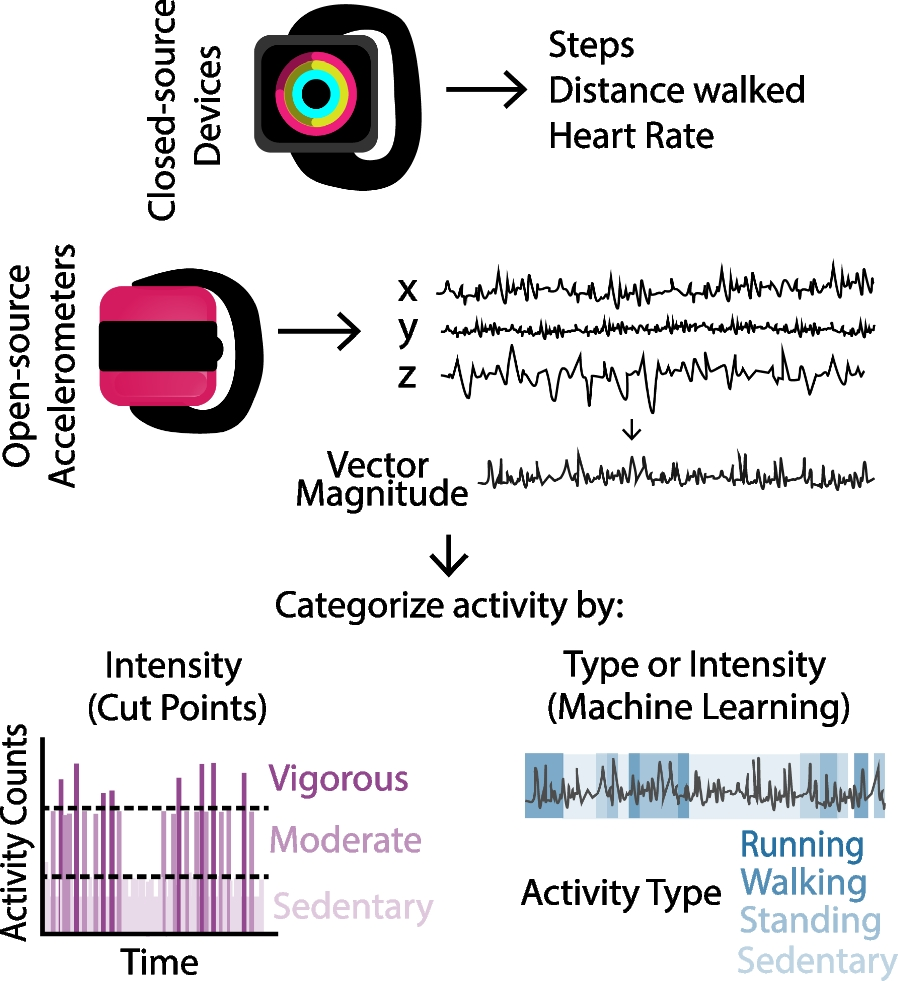
Additional force–length-velocity properties

Preliminary results using the Hill muscle model (original model, shown in orange in Fig. 3) indicated that none of the implemented and calibrated approaches accurately captured the experimental MTU force–length and force–velocity relationships. This discrepancy was observed across both dynamic and isometric protocols, with two eccentric and two concentric MVCs highlighted in red and six isometric MVCs in green in Fig. 3. Two key observations emerged:

a.

The experimental measurements and previous findings in [49] indicate that concentric contractions are most affected by musculotendon length-velocity shortening effects, whereas eccentric and isometric measurements show similar behavior. At a 60° elbow flexion angle, despite identical musculotendon lengths and moment arms, the maximum force generated during the concentric MVC was 40% lower than that of the eccentric and isometric MVCs due to the force–velocity relationship.

b.

The maximum possible value of \(f_ (v^ )\) during eccentric task, is typically set to 1.4 for young adults [50]. Given that \(f_ (0) = 1\) during isometric task, as spotlighted in Fig. 3 with the original model, the eccentric maximum forces should theoretically be 40% higher. However, neither our experimental measurements nor the results at different speeds reported in [49] confirmed this increase at the elbow joint.

Fig. 3

Preliminary comparison of the estimated torques from the original and adjusted models with experimental measurements for a healthy subject during DYN and ISOM6

As a result, the following two model adjustments were implemented to enhance MTU force estimation:

a.

With its default parameter values, the Hill muscle model failed to accurately capture the MTU force-length and force-velocity relationships, even after scaling \(l_^\), as the formulation of \(f_ (v^ )\) did not accurately represent the force-velocity dependency. The force-velocity relationship is expressed in terms of the normalized MTU fiber velocity \(\widetilde^\), which is defined as:

$$\widetilde^ = \frac }} }}$$

(11)

where \(v_\) is the maximum contraction velocity, calculated as \(v_ = \frac^ }} }}\). The parameter \(\tau_\) is known as the time-scaling parameter, and is tipically set to 0.1 s for all MTUs [32].

However, by adjusting \(\tau_\), the authors observed significant improvements (represented in brown in Fig. 3). Therefore, they decided to include this parameter in the subject-specific optimized calibration.

b.

After the first adjustment, the simulation of the dynamic task showed a good match with experimental data; however, isometric tasks were significantly underestimated, since \(f_^\) = 1.4. Therefore, we opted to set \(f_^ = 1.01\), which resulted in a stronger correlation for both dynamic and isometric tasks.

To highlight the impact of these adjustments, they were exclusively applied to a single calibration strategy—PHYS3-DYN, detailed in Sect. "Muscle force evaluation without fatigue"—rather than implementing them across all simulations.

Muscle fatigue parameters

As detailed in [29], the parameters FS and FL define the fatigue rates, while RS and RL define the recovery rates of the short-term and long-term fatigued states, respectively. Additionally, r acts as a multiplier to enhance recovery during rest. The short-duration protocol of [28] was applied, using the isometric experimental measurements during the 30-s sustained MVC at 45° to calibrate the short-term fatigue state parameters (FS, RS and r). However, due to the lack of long-duration experimental measurements, the authors adopted default values for the long-term parameters, setting RL = 2e-4 and FL = 4e-4 to induce a slight long-lasting nonmetabolic fatigue.

Model-calibration combinations and evaluationMuscle force evaluation without fatigue

As observed, numerous MTU parameters can be adjusted, and various calibration strategies are possible. To determine the simplest and most efficient non-invasive technique for musculoskeletal model calibration, this study tested different approaches by combining default and calibrated MTU parameters for two muscle models. The tested approaches are categorized as follows and summarized in Table 1:

Table 1 Summary of the approaches implemented in this study

Approaches calibrated from isometric measurements:

PHYS1-ISOM1: Only \(F_^\) of the physiological Hill-musculotendon model was calibrated by applying a single scale factor to all the MTUs derived from a single isometric measurement (ISOM1, MVC at 60°).

PHYS2-ISOM6: Individual \(F_^\) and \(l_^\) for the physiological Hill-musculotendon model were calibrated using an optimization technique based on six isometric measurements (ISOM6).

STAT-ISOM6: Individual \(F_^\) for the simplified musculotendon model were calibrated using an optimization technique based on six isometric measurements (ISOM6).

Approaches calibrated from dynamic measurements:

PHYS1-DYN: Individual \(F_^\) of the physiological Hill-musculotendon model were calibrated using an optimization technique based on dynamic experimental measurements from the isokinetic calibration task, including both concentric and eccentric contractions.

PHYS2-DYN: Individual \(F_^\) and \(l_^\) of the physiological Hill-musculotendon model were calibrated using an optimization technique based on dynamic experimental measurements from the isokinetic calibration task, including both concentric and eccentric contractions.

PHYS3-DYN: Individual \(F_^\) and \(l_^\), and \(\tau_\) of the physiological Hill-musculotendon model were calibrated using an optimization technique based on the isokinetic calibration task, including both concentric and eccentric contractions. Additionally, \(f_^\) was set to 1.01 (while set to its default value 1.4 for the others approaches).

The optimization technique (fmincon, MATLAB, version R2023a, MathWorks, Natick, MA, USA) aimed to achieve the best fit between the model and experimental results by allowing \(F_^\) to vary from 50 to 150% of its original cadaver-derived value and \(l_^\) to range from 90 to 120% of its pre-scaled value. Finally, \(\tau_\) limits were set between 1/15 s and 2 s.

As an indicator, the optimizations were conducted on a computer equipped with an Intel(R) Core(TM) i7-13700KF @ 3.40 GHz processor, 32 GB of RAM, and a 2 TB SSD running Windows 10 Pro. All calibrations were performed using a single-threaded program written in Matlab, which required less than 15 s per subject. Since computational time was not a significant factor, no specific comparison was conducted.

To compare these six approaches, the root mean square error (RMSE) was calculated between the elbow torques produced by the MTU forces estimated in each approach and the experimental measurements. This evaluation was performed separately for isometric tasks (ISOM6) and dynamic tasks (DYN). A paired-sample t-test was performed for each pair of approaches to statistically compare their differences. Prior to applying the t-tests, the normality of the paired RMSE differences was verified using the Kolmogorov–Smirnov test (after standardizing the differences), and no violations of the normality assumption were detected. To control the increased risk of Type I error due to multiple comparisons, a Bonferroni correction was applied [51]. Specifically, 15 pairwise comparisons were conducted (corresponding to all combinations of 6 approaches), and each p-value was adjusted accordingly.

Muscle force evaluation with fatigue

In this work, since the evaluated task was intended to be performed at MVC, two different hypothesis were considered for simulating muscle force and fatigue during DYN-FAT:

Option (a): Assuming TL = 100% and a = 1, based on the premise that participants maintained full MVC throughout the entire exercise.

Option (b): Estimating TL and activation level a from experimental measurements, by calculating the ratio between the experimentally measured torque and the estimated maximum torque the MTUs could generate. To avoid introducing the complexity of the force-sharing problem and the need to simulate individual muscle fatigue, a uniform activation level was applied across all MTUs at the joint level.

The differences between the two approaches affected all time steps, as any variation in MTU activation or target load leads to a different muscle fatigue time history. In this study, option (a) was tested using MTU parameters previously calibrated with the STAT-ISOM6, PHYS2-DYN, and PHYS3-DYN approaches to simulate maximum force and fatigue during DYN-FAT. Then, option (b) was tested using only the PHYS3-DYN approach, which demonstrated the best performance in this study.

Muscle force evaluation with fatigue considering maximum target load (option a)

The STAT-ISOM6, PHYS2-DYN, and PHYS3-DYN approaches were applied to simulate maximum force and fatigue development during the dynamic, short-duration, high-intensity exercise (DYN-FAT). As described in Sect. "Muscle fatigue model", the muscle fatigue model was integrated into the musculotendon model to account for task-specific fatigue during dynamic movement. The generic model parameters from the previous 3CC muscle compartment model [52], which does not account for long-term muscle fatigue, were used to simulate short-term muscle fatigue. Therefore, the parameters were set as follows: FS = 0.00912, RS = 0.00094, r = 15. For the long-term fatigue component, the parameters were set to FL = 0.0004 and RL = 0.0002.

To further evaluate the effect of subject-specific calibration of the fatigue parameters, the authors combined the calibrated fatigue parameters (Sect. "Muscle fatigue parameters") with the PHYS3-DYN muscle model, resulting in a new protocol referred to as PHYS3-DYN*.

To evaluate these four calibrations, the RMSE was computed by comparing the elbow torques generated by the estimated flexor MTU forces at maximum contraction (a = 1 and TL = 100%) with the experimental measurements. Additionally, in order to highlight the effects of these discrepancies on the determination of the target load (TL), the RMSE was calculated between the expected TL (100%) and the estimated TL*, which was determined using the following equation based on the estimated torque (\(Q_^\)) and the experimental torque (\(Q_\)):

$$TL* = \, \frac }}^ }}$$

(12)

for the non-physiological approach, and,

$$TL* = \, \frac - Q_^} }}^ - Q_^} }}$$

(13)

for the physiological approach, where \(Q_^}\) is the torque generated by the passive element, so as to isolate the ratio of torques corresponding solely to the contractile element. In both cases, TL* was limited to 100% when \(Q_^ < Q_\). To provide a statistical comparison, paired-sample t-test was also performed for each pair of approaches to statistically compare their differences.

Muscle force evaluation with fatigue from estimated target load (option b)

To assess the accuracy of the best of the previous approaches (PHYS3-DYN) in a scenario where TL is not predefined (option b) and remains unknown, we used the estimated target load based on torques proportion (TL**) to determine the corresponding MTU activations (a = TL**/100). A uniform activation level was applied across all MTUs at the joint level to avoid introducing the force-sharing problem and the need to simulate individual muscle fatigue. TL** was calculated similarly to TL* (Eq. 13), but it reflects the fatigue time history specific to this scenario. The corresponding torques and fatigue levels were computed at each time step. The RMSE was then calculated by comparing the elbow torque generated by the estimated MTU forces with the experimental measurements.