For this analysis, we employed data from the National Health and Nutrition Examination Survey (NHANES) spanning the years 2005 to 2018. NHANES is an annual data collection program run by the National Center for Health Statistics (NCHS) of the United States. It employs a nationally representative sample of non-institutionalized civilians in the United States to gather information on various health and nutritional indicators. The survey is subject to review and approval by the Disclosure Review Board of the National Centre for Health Statistics [27].

NHANES employs a random, stratified, complex, multistage sampling method. The survey encompasses health status, health care utilisation, lifestyle risk factors, prevalent diseases, and other pertinent health issues. Trained investigators conducted personal interviews to collect the required data. See https://www.cdc.gov/nchs/nhanes/index.htm for full details.

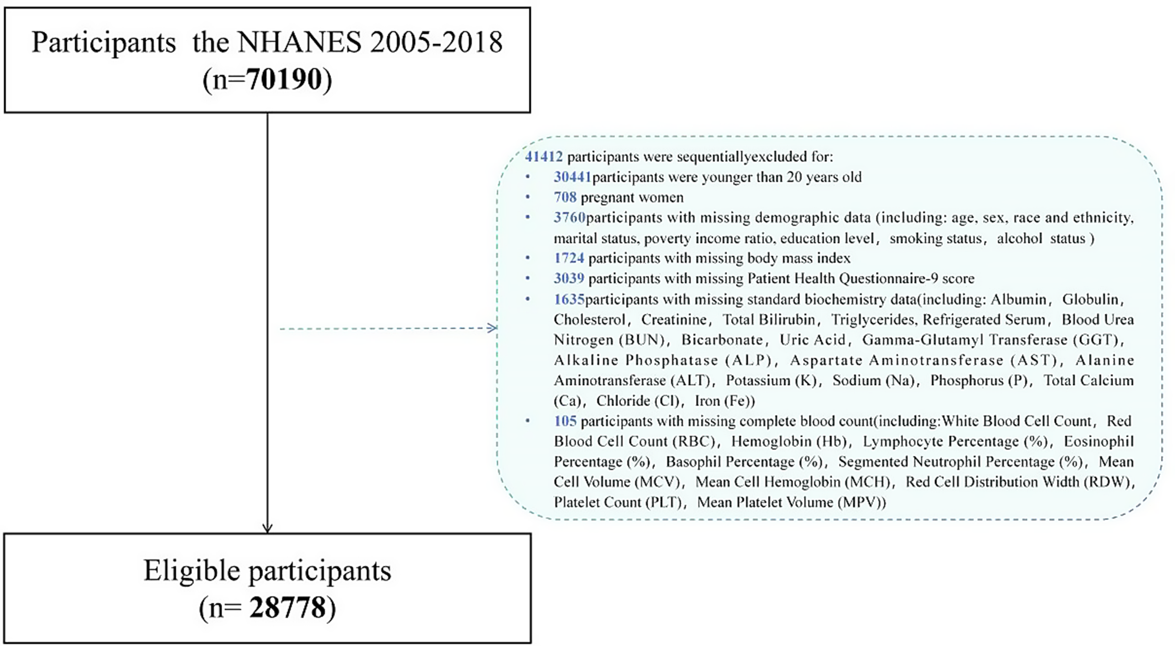
The exclusion criteria that were applied are outlined below: Of the 70,190 participants that were included in the study, the following were sequentially excluded: (1) 30,441 participants under the age of 20; (2) 708 pregnant women; (3) 3,760 participants with missing demographic data (including: age, sex, race and ethnicity, marital status, poverty income ratio, education level, smoking status, smoking status, alcohol status); (4) 1724 participants with missing body mass index; (5) 3039 participants with missing the Patient Health Questionnaire-9 (PHQ-9) score; (6) 1635 participants with missing standard biochemistry data (including: Albumin, Globulin, Cholesterol, Creatinine, Total Bilirubin. Triglycerides, refrigerated serum, blood urea nitrogen (BUN), bicarbonate, uric acid, gamma-glutamyl transferase (GGT), alkaline phosphatase (ALP), aspartate aminotransferase (AST), alanine aminotransferase (ALT), potassium (K), sodium (Na), phosphorus (P), total calcium (Ca), chloride (Cl). Iron (Fe); (7) 105 participants with incomplete complete blood counts (including: white blood cell count, red blood cell count (RBC), haemoglobin (Hb), lymphocyte percentage (%), eosinophil percentage (%), basophil percentage (%), segmented neutrophil percentage (%), mean corpuscular volume (MCV), mean corpuscular haemoglobin (MCH), red cell distribution width (RDW), platelet count (PLT), mean platelet volume (MPV)). Consequently, a total of 41,412 participants were excluded, resulting in a final analytical sample of 28,778 participants (Fig. 1).

Flowchart of the population included in our study

The severity and diagnosis of depressive episodes were determined using PHQ-9, a widely used self-report tool for depression screening. The tool consists of nine items designed to assess depression experienced during the previous two weeks. Furthermore, the measure incorporates the Diagnostic and Statistical Manual of Mental Disorders, 4th Edition (DSM-IV) diagnostic criteria for depression, as outlined therein [28].

While the PHQ-9 is based on DSM-IV diagnostic criteria, it does not exclusively capture individuals with depression but also identifies patients with other psychiatric conditions. In this study, a PHQ-9 score of 10 or more was used to define clinically significant depression. The cutoff for severe depression was set as a PHQ-9 score of 15 or more, while moderate depression was defined by a score between 10 and 14. Classification of depressive symptoms based on a PHQ-9 threshold score of 10 or more, with a total score of more than 10 defined as a clinically severely depressed patient, a threshold that is frequently employed to diagnose depression in clinical and epidemiological studies and has been clinically validated with a sensitivity of 88% and a specificity of 88% [28]. Depressive symptom scores were divided into five hierarchical categories: none (score, 0–4), mild (score, 5–9), moderate (score, 10–14), moderately severe (score, 15–19), and severe (score, ≥ 20). A binary classification of depressive symptoms was defined as a score of 10 or more [28].

The NPAR value is calculated by taking the percentage of neutrophils (as a part of the total WBC count) (%), multiplying it by 100, and then dividing the result by the level of albumin (measured in grams per liter, g/L). Haematological parameters were measured according to the NHANES CBC profile using the Beckman Coulter Automated Hematology Analyzer DxH 900 (Beckman-Coulter, Brea, CA, USA), which measures red and white blood cell counts, haemoglobin, hematocrit, and erythrocyte indices.

To assess the relationship between NPAR and depression independently, we accounted for various potential confounding factors such as age, gender, ethnicity, marital status, education level, poverty-income ratio (PIR), smoking and alcohol consumption histories, BMI (in kg/m²), and examination outcomes.

Information on the participants’ smoking and drinking status was obtained from the questionnaires used for this purpose. The questionnaires also included questions on the participants’ BMI. Regarding examination measurements, standard biochemistry data (including: Globulin, Cholesterol, Creatinine, Total Bilirubin, Triglycerides. Refrigerated Serum, Blood Urea Nitrogen, Bicarbonate, Uric Acid, Gamma-Glutamyl Transferase, Alkaline Phosphatase, Aspartate Aminotransferase, Alanine Aminotransferase, Potassium, Sodium, Phosphorus, Total Calcium, Chloride, Iron); Complete blood count (including White blood cell count, Red blood cell count, Haemoglobin, Lymphocyte percentage (%), Eosinophil percentage (%). Basophil percentage (%), mean cell volume, mean cell haemoglobin, red cell distribution width, platelet count, mean platelet volume).

In addition to the odds ratios (ORs), we have calculated the effect sizes (R-squared values) for the regression models to assess the explanatory power of the models. In the weighted logistic regression models, we adjusted for several potential confounders, including age, sex, race, BMI, smoking, alcohol consumption, and other relevant covariates. The outcome variable was depression risk, defined as either a binary classification (depressed vs. not depressed) or categorized by depression severity. We used two-year weights from the Medical Examination Component and adjusted the weights for the full 2005–2018 dataset by dividing the two-year weights by 7 to account for the seven cycles included in our analysis (i.e., 1/7×WTMEC2YR), which accounts for the complex sampling methodology. Weighted samples were generated in accordance with the analytical guidelines published by the NCHS.

We conducted subgroup and interaction analyses to test the robustness of the results across different participant groups. Given that the NHANES data employs a complex, multistage sampling approach, the missing data were assumed to be Missing Completely at Random (MCAR). Therefore, we used complete case analysis (CCA) in which observations with missing values were excluded. To ensure the robustness of our results, we conducted Little’s MCAR test and applied the multiple imputation (MICE) method for variables exceeding the missingness threshold. Additionally, we applied Restricted Cubic Spline (RCS) to model non-linear relationships. We used RCS regression models to test for non-linear associations between NPAR and depression. The RCS model was fitted using four knots, selected based on data-driven methods. Specifically, we used the Akaike Information Criterion (AIC) to determine the optimal number of knots, balancing the ability to capture nonlinear associations while minimizing the risk of overfitting. The fit of the model was evaluated using likelihood ratio tests, which compared the linear model with the non-linear RCS model to determine the most appropriate model for the data. We did not impose any constraints on the degrees of freedom for the RCS models. However, we ensured that the model did not overfit the data by selecting an appropriate number of knots and evaluating the model fit through likelihood ratio tests.

Before performing regression analysis, we tested the statistical assumptions for the models. Data distribution was assessed for normality using the Shapiro-Wilk test, and multicollinearity was examined using the Variance Inflation Factor (VIF) to ensure that no highly correlated predictors were included in the models. No significant multicollinearity was found (all VIF values were below 5), indicating that multicollinearity was not a concern.

Subgroup analyses were conducted based on demographic factors (e.g., age, gender, race) and clinical factors (e.g., smoking, alcohol use, BMI). Specifically, we stratified participants by age groups (20–45, 45–60, 60–70, 70 + years), gender (male, female), race (non-Hispanic White, non-Hispanic Black, Mexican American, etc.), education level (less than 9th grade,9-11th grade, high school grad/GED, etc.), poverty-to-income ratio (high income, low income, middle income), marital status (married, widowed, divorced, etc.), smoking, alcohol consumption, and BMI. Interaction terms between NPAR and other variables (e.g., gender, age) were included in the logistic regression models. These terms were tested using likelihood ratio tests to assess whether the effect of NPAR on depression risk varied by these factors. The significance of the interaction terms was interpreted based on p-values < 0.05. Both continuous and categorical models were used to assess the relationship between NPAR and depression to explore different aspects of the data. The continuous model treated NPAR as a continuous variable, while the categorical model divided participants into quartiles to investigate potential non-linear relationships [29,30,31]. To control the risk of false-positive findings due to multiple comparisons, we applied the Benjamini-Hochberg correction method. This method helps to control the false discovery rate across the multiple tests conducted in the study. The p-values reported in the results are adjusted for multiple comparisons. In the first quantile (Q1), “Ref.” refers to the reference group used for comparison in the logistic regression models. Three models were calculated to evaluate the robustness of the results. Model 1 was unadjusted, Model 2 adjusted for age and sex, and Model 3 included full adjustment for additional confounders such as smoking, alcohol use, and biochemical markers. The cutoffs for NPAR were determined based on the distribution of NPAR values in the dataset, with quartiles used to define the categories. These cutoffs were chosen to reflect the natural distribution of NPAR values within the population. The asymmetry in the age strata reflects the distribution of participants in the NHANES dataset, where certain age groups (e.g., 20–45 years) are more represented than others. This was an inherent characteristic of the NHANES sampling design. A “statistically significant association” is now used when the p-value is less than 0.05, while a “trend” is used when the p-value is between 0.05 and 0.10, but not statistically significant.