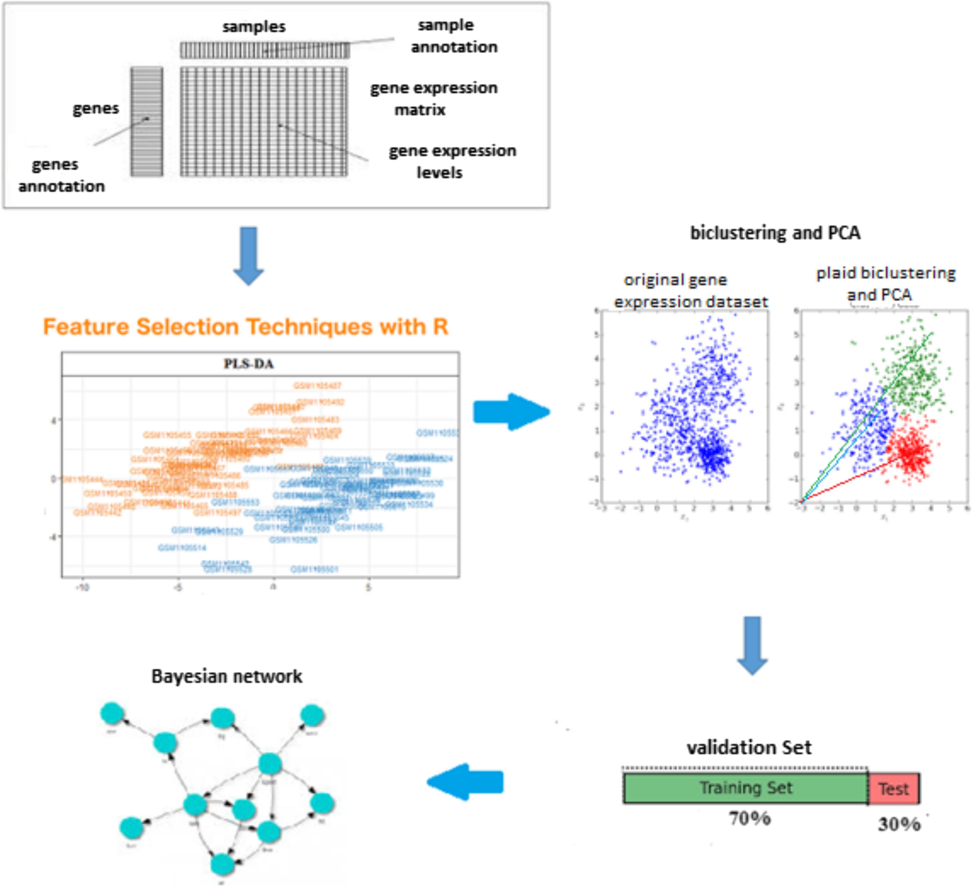
This study’s general steps of feature extraction and data classification are as follows (Fig. 1).

Fig. 1

The steps of classification of gene expression data of lithium treatment patients with BD. Gene expression data preprocessing; examining the normality and dispersion of the data. Selection of a set of genes containing information; removal of neutral and unchanged genes; biclustering of data: discovering gene sets with the same patterns using the plaid algorithm. Cluster representative selection: using principal component analysis to select a representative. Classification of data: using the DBN model. Evaluation and validation: using ROC curve analysis

Data resources

The gene expression dataset consisted of 47,323 genes and 60 patients, 32 of whom received standard treatment and 28 who underwent lithium therapy. This dataset, obtained through Affymetrix analysis, is available for download from the GEO website under the name GSE45484. Among these patients, four individuals in the control group and nine in the treatment group responded to the therapy [18]. This data set was initially analyzed by Beech et al. The study aims to classify patients based on genes whose expression in peripheral blood may serve as early markers for response to lithium treatment in patients with BD. Although changes in peripheral blood gene expression may not be directly linked to mood symptoms, biochemical variations in treatment response could obscure some heterogeneity in clinical outcomes [19].

Feature selection

The negative aspect of data generation technologies is the inclusion of irrelevant variables. Irrelevant variables can reduce model performance, increase complexity, and reduce the understanding of appropriate relationships. Therefore, removing irrelevant variables is very important [20]. To address, the large number of variables with small sample size problem that inherent in high-dimensional data sets, Partial Least Squares (PLS) regression was used in the study. This method is a supervised method developed to solve the prediction problem in multivariate problems. The variable importance in projection (VIP) index was also employed to select the most relevant variables for the model [20, 21].

Identifying genes representativePlaid biclustering algorithm

Use the bicluster algorithm to focus on a reduced set of genes for the Bayesian network analysis. Biclustering is particularly effective in datasets with varying patterns or noise levels across different groups, as it allows for filtering out noise and irrelevant features, focusing only on the clusters representing significant relationships. Biclustering leads to cleaner data, which can improve the performance of classification algorithms, allowing for the identification of subsets of data that exhibit similar behavior across conditions. Biclustering is a targeted approach that simplifies the analysis by identifying significant relationships between genes and conditions that might be missed in global analyses.

Plaid algorithm [22, 23] is a statistical model designed to detect biclusters in gene expression data by modeling the observed data matrix as a combination of multiple biclusters. It is particularly useful for uncovering overlapping patterns among a group of variables (genes) across different conditions or samples. This statistical model assumes that the level of matrix entries is a sum of a background and k biclusters. Thus, the expression matrix with I genes (Rows) and J conditions (Columns) is represented as:

$$Y_ = \mu_ + \mathop \sum \limits_^ \theta_ \rho_ \kappa_$$

where \(\mu_\) represents the general matrix background, \(\theta_ = \mu_ + \alpha_ + \beta_\), \(_}}\) is the background for bicluster k, and \(\alpha \,\,\,}\,\,\,\beta\) are column-specific additive constants in bicluster k. The variables \(\rho_ \in \left\ \right\}\) and \(\kappa_ \in \left\ \right\} \) represent gene-bicluster membership and condition-bicluster membership indicator variables, respectively. The general biclustering problem is now formulated to find parameter values so that the resulting matrix would fit the original data as much as possible. The goal of the biclustering process is to minimize the difference between the observed data and the reconstructed matrix:

$$\mathop \sum \limits_ \left[ - \sum \theta_ \rho_ \kappa_ } \right]^$$

Principal component analysis

After selecting the biclusters to determine the homogeneous and identical patterns in the selected genes, the representative of each cluster was discovered based on the principal component analysis (PCA) method [24]. PCA is a widely used statistical technique for dimensionality reduction that transforms a dataset into a new coordinate system. In this system, the greatest variance by any projection lies on the first coordinate (the first principal component), the second greatest variance on the second coordinate (the second principal component), and so on.

Suppose that the vector X contains p random variables, and there is a correlation between these p random variables. Although principal component analysis does not ignore covariances and correlations, it focuses on variances. The first step is to find a linear function of the elements of \(}\), \(}_^}} }\), that has the largest variance. The vector \(}_\) contains the constants \(a_ ,a_ , \ldots ,a_\) and

$$}_^}} } = a_ X_ + a_ X_ + \ldots + a_ X_ = \mathop \sum \limits_^ a_ X_$$

Next, the linear function is found, such that it is uncorrelated with \(}_^}} }\) and has the largest variance. This continues until, in the kth step, the linear function is found, such that \(}_}}^}} }\) has the largest variance under the condition of being uncorrelated with \(}_^}} }, }_^}} }, \ldots , }_} - 1}}^}} }\). The kth variable \(}_}}^}} }\) obtained is the kth principal component. Up to p principal components can be found, but in general, it is hoped that the largest dispersion in \(}\) remains with m principal variables (m ≤ p). To find the principal components, the random vector \(}\) is assumed to have a known covariance matrix Σ. A more realistic case is when Σ is unknown, in which case we use the sample covariance matrix S instead of the matrix Σ. For k = 1, 2,…, p, the kth principal component is given by \(Z_ = }_}}^}} }\), where a_k is the eigenvector of Σ corresponding to its kth largest eigenvalue \(\lambda_\).

Gene-ontology

Due to the large volume of information and the naming of millions of genes, researchers faced problems such as heterogeneity of terms used by different biologists and a lot of wasted time in matching information and terms. To overcome these problems, the Gene Ontology Project was founded in 1988 by genome researchers. The Gene Ontology (GO) Project provides three categories of structured and controlled terms for the interpretation of genes and gene products and attempts to standardize the naming of genes. This project describes gene products independently based on the terms biological process, molecular function, and cellular component, where:

1.

Biological process (BP): Functions or sets of molecular events with a defined beginning and end, related to the functioning of cells, tissues, and organisms.

2.

Molecular function (MF): Describes activities such as binding or catalytic activities that occur at the molecular level.

3.

Cellular Component (CC): Describes parts of a cell or extracellular environment.

To validate the findings from the biclustering analysis, existing genomic databases, such as GEO, were used. Gene enrichment analysis, a powerful computational method, was used to determine whether the identified gene sets showed statistically significant differences in expression levels or other characteristics compared to a background set of genes. This analysis is particularly valuable in understanding biological processes, pathways, or functions associated with a given set of genes of interest, such as those identified in a genomic study [25]. We performed gene enrichment analysis in the Bioconductor package.

Cross-validation

Incorporating cross-validation into the classification methods was essential for enhancing the reliability of the results, ensuring that the findings were not overfitted to the training data and could be generalized to new patients. In this study, the data were split, with 70 percent allocated to the training set and 30 percent to the test set. Given the small and sparse nature of the dataset, bootstrapping, a robust resampling technique, was employed for holdout validation. A total of 500 bootstrap samples were generated. For each bootstrap iteration, the data were randomly sampled with replacement to create a bootstrap sample, while a proportion of the data (30%) was set aside as a holdout set without replacement. The remaining data were used to train the model. The chosen classification model was fitted for each bootstrap sample, and performance was evaluated on the holdout set. Performance metrics across all bootstrap iterations were collected, and the mean and standard deviation of each metric were computed to assess overall model performance and variability.

Dirichlet Bayesian network model

We used R3.6.2 software for data analysis, and Bioconductor, Biclust, bnlearn, ropls, pROC, and Bayesian Network software packages were used.

A Bayesian network is called a directed graph (DAG), where the vertices represent random variables, and the directed edges denote the dependencies between those variables. The parameters of the network, represented as conditional probabilities, convert this structure from a qualitative state to a quantitative state. The parameters in the network determine the degree of this dependence. The Bayesian network allows for the modeling of causal relationships and is intuitively understandable due to its graphical structure.

A Bayesian network consists of two parts: Bayesian structure and Bayesian probability. The structure of Bayesian networks does not have a directed circuit, and Xi can be arranged so that the ancestors of Xi are in the set and its descendants are in the set , so according to the law of total probability, the joint probability function can be written as follows:

$$P\left( \right) = \mathop \prod \limits_^ P\left( |X_ , \ldots ,X_ } \right) = \mathop \prod \limits_^ P\left( | \prod X_ \,\,}} \right)$$

Learning the Bayesian network for data typically involves a Bayesian approach, and by using a score-based structure, the goal is to find a network for \(\varpi\) that has the highest posterior distribution probability \(\left( }\varpi } \right)\), when D is a sample from X.

$$\begin & p\left( \right) = \mathop \prod \limits_^ P\left( | \prod X_ \,\,}} \right) \\ & \,\,\, = \mathop \prod \limits_^ \left[ |\prod X_ \,\,},\, \theta } \right)P\left( }} \right)}\theta } \right] \\ \end$$

When using a Dirichlet conjugate prior, the posterior distribution remains Dirichlet, and it is computed as follows:

$$\begin & BD\left( \right) = \mathop \prod \limits_^ BD\left( |\prod X_ }; a_ } \right) \\ & \quad = \mathop \prod \limits_^ \mathop \prod \limits_^ }} \left[ } \right)}} + n_ } \right)}}\mathop \prod \limits_^ }} \frac + n_ } \right)}} } \right)}}} \right] \\ \end$$

where \(r_\) represents the number of the status of \(x_\), \(q_\) is the number of possible values of \(\prod X_ }\) that are assumed to be 1 if Xi has no ancestors, and a is Dirichlet parameter [26].

Comparative analysis of classification models

Finally, we compared the performance of DBN models with SVM and RF algorithms in various classification tasks. Each model has unique strengths, making them suitable for different applications.

Overview of SVM

SVM is a supervised learning model used to find the optimal hyperplane that separates data points of different classes in a high-dimensional space. The main goal is to maximize the margin between the closest data points of each class, known as support vectors, which helps improve classification performance. For a binary classification problem, the decision function of an SVM can be expressed as:

$$f\left( x \right) = w \cdot x + b$$

where w is the weight vector (normal vector to the hyperplane), x is the feature vector of the input data, and b is the bias term, which determines the hyperplane's offset from the origin. SVM aims to maximize the margin between the two classes. The optimization problem can be formalized as minimizing:

subject to the constraints \(y_ \left( + b} \right) \ge 1\). Here, yi represents the class label for each data point xi, which takes values of + 1 or − 1 [27].

Overview of RF

RF is a robust ensemble machine learning algorithm combining multiple decision trees to improve prediction accuracy and robustness in classification and regression tasks. RF begins by selecting random samples from the training dataset. This sampling is done with replacement, meaning some data points may be repeated while others may be omitted. For each sample, a decision tree is constructed. During the creation of each tree, only a random subset of features is considered for splitting at each node. This randomness helps ensure that the trees are uncorrelated. For classification tasks, each tree makes a prediction (votes for a class label), and the class with the majority votes becomes the final prediction. This ensemble approach allows Random Forest to mitigate the risk of overfitting common in individual decision trees, leading to better generalization on unseen data[28].

Performance of the classification model

The Receiver operating characteristic (ROC) curve plots the true positive rate (sensitivity) against the false positive rate [1-specificity] at various thresholds, providing a graphical representation of the trade-off between sensitivity and specificity. The ROC curve helps choose a threshold and evaluate the trade-off between sensitivity and specificity.

The Area under the Curve (AUC) summarizes the overall ability of the model to discriminate between the classes; a higher AUC indicates a better-performing model. This metric is particularly useful for comparing the performance of different models, as it considers performance across all possible classification thresholds [29].