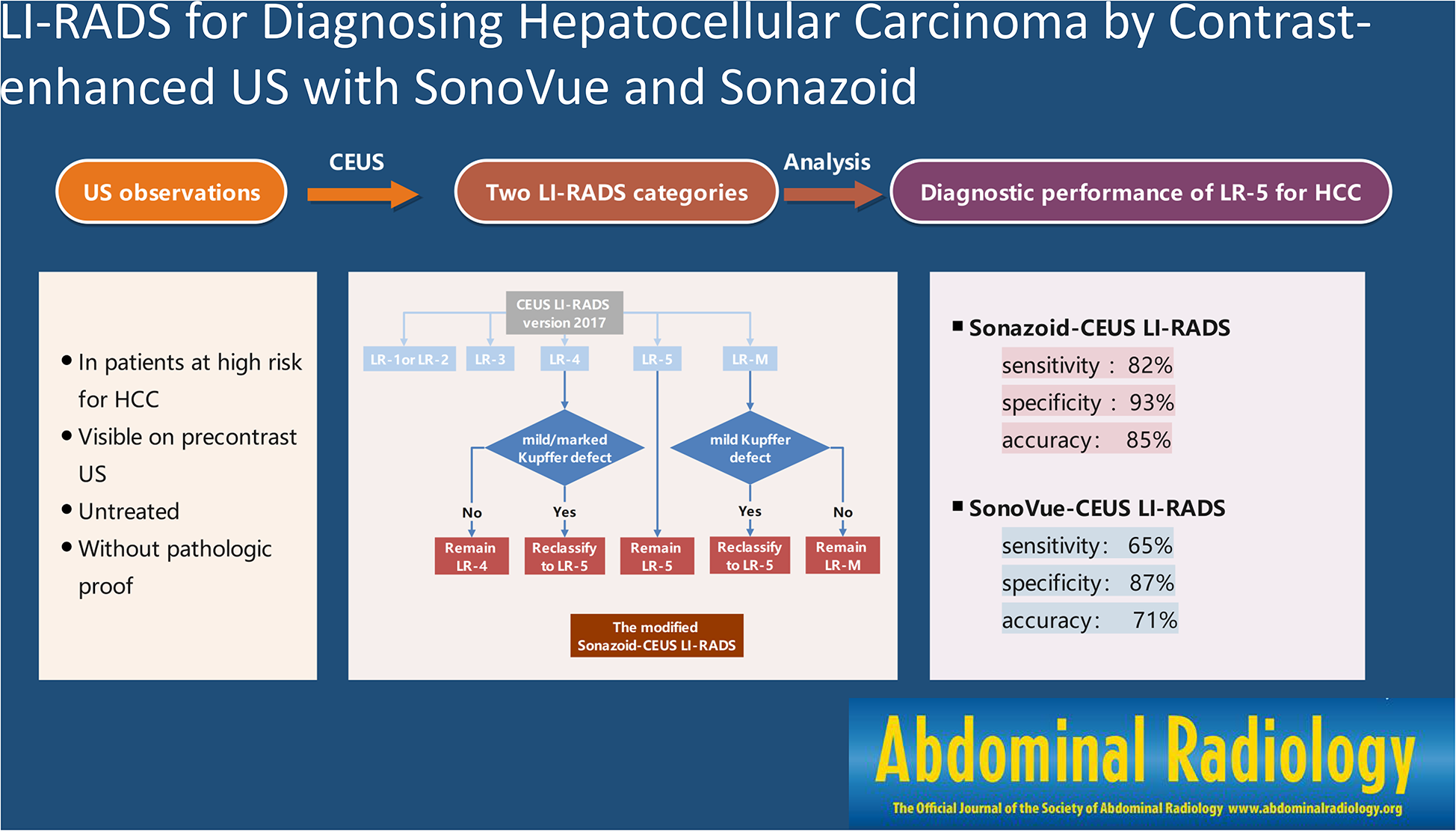
This single-institution prospective study with healthy volunteers received approval from Champalimaud Foundation Ethics Committee (project “DWI-P”), and each participant gave a fully informed consent before undergoing MRI.

Healthy volunteers were recruited from the Institution’s staff and in an opportunistic way from visitors to the Institution.

Inclusion criteria were people aged 18 to 65 years-old, healthy, willing to participate and undergo MRI.

Volunteers with history of any pancreatic disease (acute or chronic pancreatitis, auto-immune pancreatitis, pancreatic exocrine insufficiency, Diabetes Mellitus, pancreatic tumors) were excluded from the study. Volunteers with contraindications for MRI, including claustrophobia or incompatible medical devices, were also excluded from the study.

Each participant underwent MRI in a clinical 3T scanner (Ingenia®, Philips NV, The Netherlands) with a 16-channel phased-array body coil. Participants were instructed to fast for at least 4 h before MRI.

The acquisition included a T2-weighted Turbo Spin-echo (TSE) in the axial plane, for pancreatic anatomical definition. For DTI and DKI, a 2D Spin-echo Echo-planar-imaging (SE-EPI) was acquired with 6 slices encompassing the entire pancreas, with the following b values: 0, 200, 1000 and 1700 s/mm2 [21]. The complete parameter list is found in Table 1.

Two different diffusion direction protocols were tested: 16 and 6 evenly diffusion directions. The first protocol with 16 directions was aimed at providing a more robust representation of the diffusion tensor, while also providing redundant data for a more effective denoising, while sacrificing acquisition time length [22,23,24]. The second protocol with 6 directions provided a significantly faster acquisition, however with the minimum number of directions required for estimating the diffusion tensor, and with less redundant data for the denoising algorithm [23]. Scan lengths were recorded for comparison, as acquisition time was variable due to respiratory triggering.

Acquisitions were repeated twice in the same scanning session, in order to assess intra-subject repeatability.

Datasets were analyzed using in-house developed code in MATLAB™ (MathWorks Inc., Natick, MA). Pre-processing included denoising based on Marchenko-Pastur principal component analysis (MP-PCA) and Gibbs unringing algorithms [24, 25].

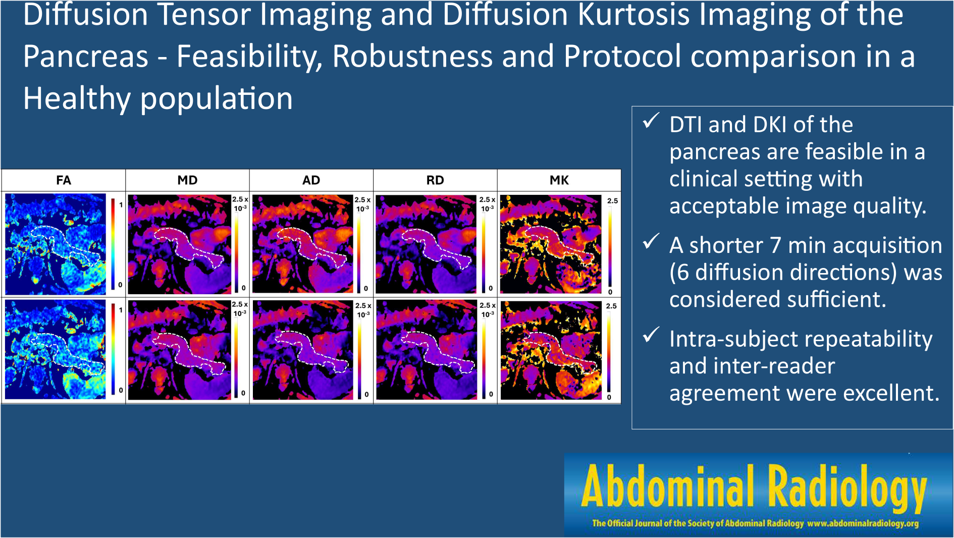
DTI was fitted per voxel with a weighted-least-squares solution as described by Veraart, et al., using the acquired b values of 200 and 1000 s/mm2 for removing perfusion-related effects [21, 26, 27]. This first calculation provides for each voxel a six-parameter tensor, from which three principal eigenvectors can be extracted, each with a corresponding eigenvalue. These eigenvalues (λ1, λ2, λ3) numbered from largest to lowest, represent the three orthogonal diffusion coefficients in the diffusion frame of each voxel. From these diffusion coefficients, mean diffusivity (MD), axial diffusivity (AD), radial diffusivity (RD) and fractional anisotropy (FA) maps were produced, for each acquisition of each volunteer. MD was calculated as the average diffusion coefficient, as follows:

$$\:MD=\:\frac}_+\:}_+\:}_}$$

AD, the largest diffusion coefficient of each voxel was equal to λ1. RD was calculated as the average of the two smaller diffusion coefficients:

FA, quantifying the amount of diffusion anisotropy in each voxel, was calculated as previously described [28]:

$$FA = \sqrt } - MD} \right)}^2} + - MD} \right)}^2}} \right.} \\ - MD} \right)}^2}} \right)/\left( ^2 + ^2 + ^2} \right)}\end} $$

DKI was fitted to the directional averaged acquired data using b values of 200, 1000 and 1700 s/mm2. The full details for DKI fitting in directional averaged signals are described in [29, 30], however, in short, mean signals for each b value are computed as the average from all directions before fitting. Then, the DKI model is fitted using a weighted linear least squares solution of the following expression:

$$\:MS\left(b\right)\approx\:_^^^MK)}$$

Here, MS represents the directional averaged diffusion-weighted signal for each b value, S0 the non-diffusion-weighted signal, MD is the mean diffusivity and MK the mean kurtosis. MK maps were then produced for analysis, for each acquisition for each volunteer.

ADC maps were produced for comparison as in standard clinical practice, using a monoexponential fit with b values of 200 and 1000 s/mm2:

Where S represents the measured diffusion-weighted signal for a given direction. Only the first diffusion direction was used to calculate ADC, as in clinical practice, following the isotropic diffusion principle assumed by the conventional unidirectional model of DWI.

Two abdominal radiologists, with 11 and 13 years of experience, delineated the entire pancreas in each slice using MATLAB™’s built-in segmentation tools, on b = 0 s/mm2 images and supported by the T2-weighted images. The resulting Regions of interest (ROI) were then placed in the corresponding ADC, FA, MD, AD, RD and MK maps, for extracting quantitative data.

Measurements from each reader were compared to assess inter-reader variability. Measurements from each volunteer, regarding the two repeated acquisitions, were compared to assess intra-subject repeatability.

The results from each protocol (16 and 6 diffusion directions) were compared for each map. Besides median values and range comparisons, the 90th and 10th percentiles of the DTI, DKI and ADC maps were also extracted from each participant, in order to provide a more granular analysis of extreme measurements. Finally, a measurement of excluded voxels with implausible values due to artifactual results (i.e. negative diffusivity/kurtosis values, kurtosis values larger than 2.5, FA and diffusivity values larger than 1) was compared between each protocol for each map to assess if any of the protocols was more robust in terms of artifactual measurements. The > 2.5 cutoff for implausible positive MK estimates was selected on the basis of previous findings [14, 18, 20, 31, 32]. The preliminary MK estimations in our subjects also contributed to selecting this cutoff, as MK values > 2.5 were only rarely observed as outliers.

For subjective image quality assessment, each DTI and DKI map (FA, MD, AD, RD, MK and ADC) were classified by each reader using an adapted Likert scale from 1 (worst) to 5 (best), for the following parameters: anatomical delineation, image graininess, distortion artifacts, motion artifacts (Table 2). Ghost artifacts were also searched for but were not evident in our images, and were thus excluded from this analysis.

IBM SPSS® statistics v.24 was used for statistical analyses. The Kolmogorov-Smirnov was used to assess the normality of distribution of continuous variables, revealing not all tested variables had a normal distribution. We thus opted for non-parametric tests: Mann-Whitney’s U test was used to compare groups of continuous and ordinal variables; Fisher’s exact test was used for comparing categorical variables.

Bland-Altman analysis was used to assess intra-subject repeatability, and the coefficient of repeatability (r) was calculated according to [33, 34]:

$$\:r=1.96*\sqrt^$}\!\left/\:\!\raisebox\right.}$$

Where d is the difference between acquisitions and n the number of volunteers.

Intraclass correlation coefficient was used to assess inter-reader agreement for pancreatic quantification in each map, as follows: <0.5 considered poor, 0.5 to 0.75 considered moderate, 0.75 to 0.9 considered good, > 0.90 considered excellent [35]. For subjective image quality comparisons, weighted Kappa was used to assess inter-reader agreement (quadratic form for weighting difference magnitude), and was classified as: less than chance (< 0), slight (0.01–0.2), fair (0.21–0.4), moderate (0.41–0.6), substantial (0.61–0.8), almost perfect (> 0.81) [36, 37].

p < 0.05 was considered significant.