Developing a robust Brain Age model involves several crucial steps. Firstly, it is imperative to assemble a diverse, broad, and representative dataset that encompasses neuroimaging data alongside corresponding chronological ages. The size of the dataset plays a significant role, as a larger dataset enables greater precision and generalizability in the final model. Subsequently, feature extraction is performed to capture pertinent information from the neuroimaging data. This process ensures that only informative and discriminative features are included in the model.

Once the features have been extracted, an appropriate machine-learning algorithm is selected for age prediction based on the neuroimaging data. Common choices include support vector machines or neural networks. The chosen algorithm is then trained using the dataset, and techniques such as regularization, cross-validation, and hyperparameter tuning are employed to optimize performance and prevent overfitting. The trained model is next evaluated using a separate dataset, employing metrics such as mean absolute error (MAE) or correlation coefficients to assess accuracy and generalization capabilities. This evaluation step provides valuable insights into the model’s performance and its ability to accurately estimate Brain Age.

Finally, the trained Brain Age model can be applied to new and unseen neuroimaging data. In our case, we apply it to a dataset composed of healthy controls, patients with episodic migraine, and patients with chronic migraine.

Brain age model

To create and evaluate our age prediction models, we compiled a dataset (hereinafter referred to as Model Creation Dataset) consisting of 2,771 structural T1w MRI scans from different studies and databases that were publicly available. These include: the Dallas Lifespan Brain Study (DLBS) [24]; the Consortium for Reliability and Reproducibility dataset (CoRR) [25]; the Neurocognitive aging data release (NeuroCog) [26]; The OASIS-1 dataset [27]; the Southwest University Adult Lifespan Dataset (SALD) [28]; the Information eXtraction from Images dataset (IXI) [29]; and the CamCAN repository (available at http://www.mrc-cbu.cam.ac.uk/datasets/camcan/) [30, 31]. In addition to these, we included a set of healthy adults from the Laboratorio de Procesado de Imagen (LPI), our own institution. We selected only participants in good health and within the age range of 18 to 60 years. Individuals who presented neurological or psychological diagnoses or cognitive impairments were eliminated from the OASIS-1 and CoRR databases. Table 1 depicts the basic features of the Model Creation Dataset. Supplementary file 2 offers a detailed description of the included acquisitions for each database.

Table 1 Summary characteristics of the datasets used in the Model Creation Dataset, sorted by median age

From the T1w images, FastSurfer [32] was employed to extract a total of 1,479 features. Fastsurfer uses Deep Learning to perform brain segmentation based on the Desikan-Killiany atlas [33, 34]. Two types of features were extracted:

624 morphological features, including whole brain features, the volume of cortical and subcortical gray matter regions and white matter regions from the atlas, as well as the surface, thickness and curvature of the cortical regions. This feature set will be referred to as Morphological Feature Set.

855 intensity-based features extracted from the same regions. This feature set will be referred to as Intensity Feature Set.

Together, all 1,479 features make up the Combined Feature Set. The three feature sets obtained using this procedure were the basis for further analysis.

To ensure their quality, segmentations were manually inspected. In Supplementary Table 1, Supplementary Fig. 1 and Supplementary Table 2, features and regions of interest are covered in greater detail.

MRI acquisitions obtained at different sites and/or using different protocols can differ in their intensity levels, which can introduce a bias in the Brain Age-predicting models. In order to cope with this problem, we used ComBat [35, 36] to harmonize the features from the Intensity Feature Set and the Combined Feature Set, using age, sex, and estimated total intracranial volume (eTIV) as covariates.

Afterwards, the cases were randomly divided into an 8:1:1 ratio for training, validation, and testing. We conducted a 10-fold cross-validation training procedure over the harmonized features to predict age. We flattened outliers of each feature, defined as values on the 97.5th or 2.5th percentile. In addition, each characteristic was adjusted to the range (-1, 1) using min-max normalization. Each fold underwent feature selection, defining three sets of 20, 30, and 40 characteristics. The selection of features was accomplished in two steps. Initially, a filter was used to choose the first decile features based on the mutual information between features and age in the training set. Next, the final features were chosen by employing a forward feature selection approach with gaussian mixture models to optimize the mutual information between a subset of features and age [37].

As regressors, support vector regressor (SVR), random forest (RF), and a multilayer perceptron (MLP) were evaluated. Figure 1 depicts the process followed. By combining these three regressors with distinct feature sets of 20, 30, and 40 characteristics for each fold, a total of 90 models were trained.

Fig. 1

Comprehensive illustration of the methodologies employed for the training of the Brain Age models and the generation of brain-predicted ages. Model Creation shows the steps taken to train the Brain Age model on the Model Creation Dataset and choose the final model applied on the Application Dataset: a Image processing includes Fastsurfer for brain segmentation and extraction of intensity and morphological features, thus building three feature sets: the Morphological Feature Set, Intensity Feature Set and the Combined Feature Set. For each of these feature sets, a feature selection procedure is performed in a 10-fold cross-validation scheme creating feature sets of 20, 30 and 40 features to feed the machine learning models (SVR, RF and MLP) for each fold. b Validation is performed to select the best combination of feature set size and machine learning technique. c Test on the Model Creation Dataset to assess the performance of the Brain Age prediction model. Model Application depicts the use of the chosen model on the patient and healthy groups. Brain Age Gap is calculated as the difference between the predicted and the actual age. Differences in Brain Age Gap are then analyzed

Predictions were obtained for the validation and test set for each fold. Validation results were used to select the Brain Age model to be selected as the best-performing, while test results were exclusively employed to report the accuracy of the Brain Age model on the Model Creation Dataset.

We are aware that Brain Age models suffer from regression dilution, which causes bias in Brain Age predictions. Therefore, in order to avoid possible spurious associations, a correction for this effect was applied [38, 39]. A linear regression was fitted between the real age and validation results of each of the regressors of the ensemble. The intercept \((\alpha )\) and slope \((\beta )\) of each fit were then used to correct the predictions obtained for the studied groups following the equation:

$$\begin \text = (\text - \beta ) / \alpha \end$$

(1)

This approach was repeated for each of the aforementioned feature sets. The training procedure was performed using the scikit-learn Python library for machine learning [40]. The SVR and RF models were imported from the library while the MLP was implemented using PyTorch [41]. Details of the MLP implementation and the hyperparameters for each model are described in Supplementary Table 3.

Participants

A total of 391 subjects were included in this study, on which the Brain Age model previously described was applied. First, we employed healthy subjects from the Nathan Kline Institute - Rockland Sample (NKI-RS) dataset [42], for the purpose of external validation (n = 144). Next, and in order to study the influence of migraine on Brain Age, we employed a dataset composed of healthy controls (HC, n=82), EM (n=91), and CM patients (n=74). This dataset will be hereinafter referred to as Application Dataset.

Patients were recruited from the outpatient headache unit at the Hospital Clínico Universitario de Valladolid (Spain), a public tertiary care institution that accepts patients from both secondary care and primary care. Inclusion criteria were: a) migraine diagnosis using the third edition of the International Classification of Headache Disorders (ICHD-3) beta and ICHD-3 criteria [1, 43]; b) a stable clinical state in the last six months; and c) expressed willingness to partake in the study, coupled with the voluntary signing of the informed consent document. We excluded patients with the following conditions: a) high-frequency episodic migraine, with 10 to 14 headache days per month; b) other painful conditions; c) known major psychiatric diseases (described as anamnesis or the presence of depression or anxiety in the Hospital Anxiety and Depression Scale [44]); d) other neurological diseases; e) drug or substance abuse; and f) pregnancy. At the time of inclusion, no preventive treatment was given to the patients. Participants were requested to complete a headache diary and were diagnosed with EM if they experienced 10 headache days per month or less and CM if they met the ICHD-3 criteria.

Age- and sex-matched HC were recruited through hospital and university colleagues, as well as ads at these institutions, using convenience sampling and snowball sampling. No HC were included if they had a current or previous history of migraine, or if they had any other neurological or mental disorder following the same exclusion criteria as for migraine patients.

We gathered sociodemographic and clinical data from all patients, including migraine illness duration (years) and headache and migraine frequency (days per month).

The study was approved by Hospital Clínico Universitario de Valladolid’s local Ethics Committee (PI: 14- 197). All participants read and signed a written consent form before their participation.

Image acquisition and processing

High-resolution 3D T1w MRI data were acquired for all subjects using a Philips Achieva 3T MRI unit (Philips Healthcare, Best, the Netherlands) with a 32-channel head coil in the MRI facility at the Universidad de Valladolid (Spain). Acquisition parameters were the following: Turbo Field Echo (TFE) sequence, repetition time (TR) = 8.1 ms, echo time (TE) = 3.7 ms, flip angle=\(8^o\), \(256\times 256\) matrix size, \(1\times 1\times 1\) mm\(^3\) of spatial resolution, and 160 sagittal slices covering the whole brain. Image acquisitions for migraine patients were performed during interictal periods (defined as at least 24 hours from the last migraine attack). Details about the acquisition protocols of each public dataset are described in Supplementary Table 4. If more information is required, further details can be found in each portal of the databases used.

Following the image acquisition, image segmentation, feature extraction and harmonization were also performed on the Application Dataset as described for the creation of the Brain Age model. Next, Brain Age was estimated for each participant, including correction from the regression dilution. Since we conducted a 10-fold cross-validation for the training, validation and testing of the Brain Age model, an ensemble formed with the average result of the trained model from each fold was used to obtain the final prediction. Finally, the Brain Age Gap was calculated as the difference between the corrected predicted age and the chronological age of each individual.

Model interpretation

The significance of each imaging feature in the Brain Age estimation was evaluated using SHapley Additive exPlanations (SHAP) [45]. SHAP is a game-theory-based model-agnostic explanation method for machine learning models that evaluates the contribution of each feature to a given prediction. By employing this approach, a group-level comparison of distinct brain imaging features can be conducted to determine their significant contribution to age prediction. Additionally, the evaluation of the influence of individual features on each participant’s Brain Age prediction is made possible, as exemplified in the study conducted by Ballester et al. [46].

The SHAP value for a particular feature for a specific prediction can be interpreted as the difference in the prediction when that feature is omitted from the model. SHAP values reinterpret complex models as a linear function:

$$\begin g(z') = \phi _0 + \sum \phi _i z'_i \end$$

(2)

where z’ is a simplified version of the input features of the model, \(\phi _0\) is a reference value of the model (in our case is a value close to the average age of the training data), and \(\phi _i\), the attribute effect of the feature which deviates the prediction from the reference value. In a database with N participants and M features, for example, SHAP generates an \(N\times M\) matrix, where each value represents the contribution of feature m to the prediction of participant n.

We calculated the SHAP value for each subject for a deeper understanding of the regressors. Since many features are repeated across the different regressors, we summed up the contribution of repeated features into a single value. The final matrix was divided by 10 since our ensemble model is the average of the results of the 10 regressors trained during the 10-fold cross-validation.

Once we had the final matrix, we aggregated the values for each of the groups considered (HC, EM and CM) by summing up the absolute values of the matrix along the participant’s axis. The best 15 features in terms of their absolute contribution for each group were selected for each model of the ensemble. Unique features among the three groups studied were selected as the most informative features.

Statistical analysis

The performance evaluation of the Brain Age models was conducted using two metrics: the MAE and Pearson’s correlation coefficient (r). The MAE was calculated as the average of the absolute values of the residuals, which were obtained by subtracting the predicted age from the actual age for each individual in the group. The MAE serves as a comprehensive measure of the prediction error across the entire group, with lower values indicating a better fit. On the other hand, Pearson’s correlation coefficient measures the strength and direction of the linear relationship between the predicted ages and the real ages. Higher values of r indicate a better fit of the model. The specific formulas for these metrics can be found in equations (3) and (4). Further exploration of these performance metrics can be found in the work from de Lange et al. [39].

$$\begin MAE = \frac\sum _^|\tilde_i-y_i| \end$$

(3)

$$\begin r = \frac)(\hat_i-\bar})})^2\sum (\hat_i-\bar})^2}} \end$$

(4)

We assessed the normality and homogeneity of variance for age and duration of migraine in the Application Dataset using the Kolmogorov-Smirnov test and Levene’s test for equality of variances, respectively. If the null hypothesis was not rejected in both tests, we performed a one-way analysis of variance (ANOVA) to determine significant differences in the ages of the three groups. Gender-significant differences were identified using a chi-square test. For comparing clinical characteristics between migraine patients (i.e., duration of migraine history in years for both groups of patients), we used a two-tailed unpaired t-test if the null hypothesis was not rejected by the Kolmogorov-Smirnov; alternatively, we used the Mann-Whitney U test.

An Analysis of Covariance (ANCOVA) was conducted on the Brain Age Gap outcomes across the three groups, incorporating eTIV and sex as covariates. Upon ascertaining that the p-value suggested a need for further investigation, pairwise comparisons between the groups were carried out, keeping the same covariates. The analysis was made using all subjects followed by sex-specific comparisons. To verify that the Brain Age Gap calculated for each group was approximately normal and that the variances between groups were comparable, we performed the Kolmogorov-Smirnov test and the Levene test. In the case of a negative Levene’s test, we verified that the variance ratio did not exceed 2 [47]. We reset the P value threshold correcting for multiple comparisons using the Bonferroni correction method (P threshold = 0.0167). To conduct a more detailed examination of the variations among the groups, we computed the Cohen’s d statistic.

Regarding the model interpretation, We conducted a Kruskal-Wallis test on the SHAP values obtained for each of the highly important features of each regressor trained to analyze differences in feature importance among the studied groups. A non-parametric test was chosen due to the non-normality of the SHAP values. To account for multiple comparisons, we applied the Benjamini-Hochberg correction method. We performed pairwise comparisons using the post-hoc Connover-Iman test, correcting its p-values for multiple comparisons using the Benjamini-Hochberg method if the Kruskal-Wallis Test was significant.

To deepen our understanding of how migraines influence brain health, we examined the role of brain volume in linking the frequency of headaches in migraine patients to the Brain Age Gap. This type of analysis, known as mediation analysis, is a standard method in the realm of neuroimaging [48]. Utilizing a single-tier, three-variable mediation model, we sought to discover if segmented brain volume could serve as a mediator (M) between headache frequency (independent variable, X) and the Brain Age Gap (dependent variable, Y). We adjusted for potential confounding factors like age and sex in the model. To assess the validity of the mediation effect, we employed a bias-corrected bootstrap technique, using 10,000 random samples. For a more nuanced understanding, we looked at these relationships both across the general population of migraine patients and within individual subgroups.

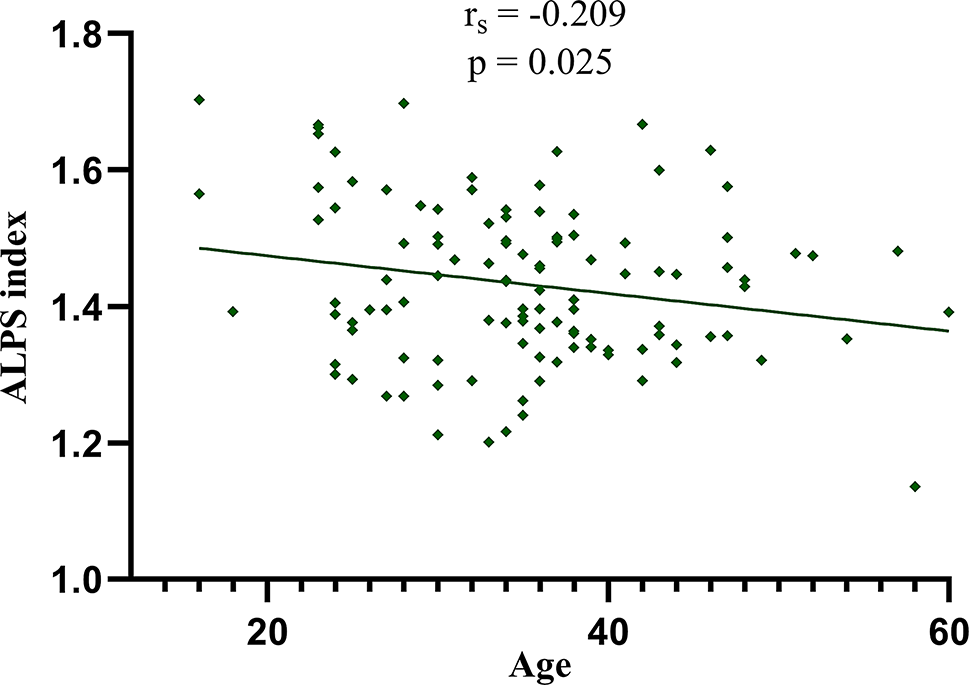
Finally, we computed the Pearson’s correlation coefficient to assess the association between the Brain Age Gap and the clinical characteristics of the migraine groups. Corrections for multiple comparisons were made using the Benjamini-Hochberg method. We also explored the relationship between the imaging features that were selected as highly important during the SHAP analysis and these clinical characteristics, making additional adjustments for multiple comparisons using the Benjamini-Hochberg approach. Partial correlation analyses were performed to control for age as a confounding variable given its potential influence on the duration of migraine and chronic migraine. All statistical procedures were executed in Python.