In this appendix we provide more details on some technical derivations.

In this section we show how to derive the true model for \(\Delta\)QTc. Let us start with assuming that the QTc data are generated from model (6) and random effects model (7). From this, one can derive the statistical model for \(\Delta\)QTc as

$$\begin Y_ = \mu ^* + \pi _t + \vartheta C_ + Z^*_ \; , \end$$

(A1)

with random effects model

$$\begin Z^*_ = U^*_ + V^*_ + R_ + S_C_ + \varepsilon _ \; . \end$$

(A2)

The terms like \(\pi _t\), \(\vartheta\), \(C_\), \(R_\), and \(\varepsilon _\) are the exact same as the corresponding ones in model (6) and random effects model (7). The terms with an asterix are new terms, and they are defined as

$$\begin \mu ^* = -\frac \sum _^ \pi _ \; , \end$$

(A3)

$$\begin U^*_ = -\frac \sum _^ R_ \; , \end$$

(A4)

and

$$\begin V^*_ = -\frac \sum _^ \varepsilon _ \; \end$$

(A5)

in the case of an interleaved design. All other terms (like \(\mu\), \(\alpha _i\), \(\beta _j\), \(U_\), and \(V_\) from models (6) and (7) disappear via subtraction).

From Eqs. A4 and A5 one can immediately derive that the variance of the random subject effect on the \(\Delta\)QTc level is \(\sigma ^2_=\frac\sigma ^2_\), and that the variance of the random subject by period interaction on the \(\Delta\)QTc level is \(\sigma ^2_=\frac\sigma ^2_\) (see Table 1).

One should specifically note that if there is no random subject by time interaction in the random effects model (7) (e.g., if \(\sigma ^2_R=0\)), then there is no random subject effect on the \(\Delta\)QTc level. Hence, a model with a random subject effect alone, but without a random subject by time interaction does not occur on the \(\Delta\)QTc level. Either both terms are there, or none. Analysis models which do not meet this condition are a priori misspecified. (One could use a random subject pre/post dose interaction instead of the random subject by time effect, but the principle remains.)

However, there is always an random subject by period interaction term on the \(\Delta\)QTc level (assuming that there is always a random noise term on the QTc data level).

This implies that the analysis model 1 is always misspecified for an interleaved design. It is either underspecified (random subject by period and random subject by time interactions are missing), or the wrong random effect is used (subject rather than subject by period interaction).

In the case of a parallel group design, there is only one period per subject and no sequences, so that the model and notation simplifies to

$$\begin X_ = \mu + \pi _t + \vartheta C_ + Z_ \; \end$$

(A6)

and

$$\begin Z_ = U_ + V_ + R_ + S_C_ + \varepsilon _ \; , \end$$

(A7)

The random subject effect and the random subject period interaction are indistinguishable, because there is only one period, and the random subject time interaction is likewise indistinguishable from the noise. To keep matters comparable in the simulations, we use a normal distribution with variance \(\sigma ^2_U+\sigma ^2_V\) for the random subject effect, and a normal distribution with variance \(\sigma ^2_R+\sigma ^2_\varepsilon\) for the noise.

On the \(\Delta\)QTc level this translates into

$$\begin U^*_ = \frac \sum _^ ( R_ + \varepsilon _)\; . \end$$

(A8)

There is no random subject by period interaction, as there is only one period per subject.

In this section we assess the impact of the random subject slope on the correlations between different periods for interleaved designs. For an individual subject, the covariance between two periods \(j_1 \ne j_2\) and a selected time point t is defined to be

$$\begin \mathbb \left[ \left( Y_-\mathbb [Y_] \right) \left( Y_-\mathbb [Y_] \right) \right] \end$$

(A9)

The expectations in Eq. A9 are to be understood conditionally on the concentrations \(C_\) and \(C_\). The periods \(j_1\) and \(j_2\) are both either odd numbers (for a subject from cohort 1) or both even numbers (for a subject from cohort 2). Using (9) one can show that the covariance equals

$$\begin \mathbb [U_^] + \mathbb [R_^] + \mathbb [S_^]C_C_ \; , \end$$

(A10)

because \(\mathbb [V_V_]=0\) and \(\mathbb [\varepsilon _\varepsilon _]=0\). This equals

$$\begin \frac\sigma ^2_R + \sigma ^2_R + \sigma ^2_S C_C_ \; , \end$$

(A11)

Note that for any pair \(j_1 \ne j_2\) there are two sequences where either \(C_=0\) or \(C_=0\) by design, so that the product \(C_C_\) equals 0 for half of the subjects in a cohort, regardless of the cohort, the periods \(j_1 \ne j_2\), and the time point t.

The conditional variance

$$\begin \mathbb \left[ \left( Y_-\mathbb [Y_] \right) ^2 \right] \end$$

(A12)

for an individual subject in period j and at time point t can be obtained correspondingly as

$$\begin (1+\frac)\sigma ^2_R + (1+\frac)\sigma ^2_\varepsilon + \sigma ^2_S C^2_ \; . \end$$

(A13)

Here, for each period j there is one sequence where \(C_=0\) by design, so that \(C^2_=0\) for one quarter of the subjects in a cohort.

Therefore, if there is no random subject slope (\(\sigma ^2_S=0\)), the correlation (conditional on the concentrations) between periods \(j_1 \ne j_2\) is

$$\begin \frac \; , \end$$

(A14)

regardless of the time point t. If \(\sigma ^2_S>0\), the correlation between periods \(j_1 \ne j_2\) at time t for an individual subject is either (with \(\phi _M:=1+\frac\))

$$\begin \frac\sqrt}} \end$$

(A15)

(if placebo is administered in period \(j_1\) for sequence i, e.g., if \(\ell (i,j_1)=0\)), or

$$\begin \frac\sqrt} } \end$$

(A16)

(if placebo is administered in period \(j_2\) for sequence i, e.g., if \(\ell (i,j_2)=0\)), or

$$\begin \fracC_}} \sqrt}} \end$$

(A17)

(if placebo is neither administered in period \(j_1\) nor in period \(j_2\) for sequence i).

Note that (A15) and Eq. A16 are both smaller than \(\frac\), so that the random subject slope reduces the correlation for a subject in these sequences as compared to a model without such a random slope. At the same time, \(\frac(1-\frac}}})\) (with \(j=j_1\) or \(j=j_2\)) is a lower bound for these two correlations (A15) and Eq. A16, because \(\sqrt+\sqrt \ge \sqrt\). This implies that the reduction in correlation can be more pronounced when the concentration \(C_\) is high (i.e., for time points around \(t_\)), and less pronounced when the concentration is low. For low concentrations, the between period correlation is expected to be more or less equal to \(\frac\), the value that applies when there is no random slope.

Note further that the correlation (A17) has an upper bound

$$\begin \frac + \dots \quad \quad \quad \quad \\ \dots + \fracC_}} \sqrt}} \; , \nonumber \end$$

(A18)

and a lower bound which is equal to

$$\begin \frac(1-\frac}}} \nonumber \\ -\frac}}}) \; . \end$$

(A19)

Again, for small concentrations (i.e., for time points which are far away from \(t_\)) the correlation between the two periods is close to the reference value\(\frac\), the value that applies when there is no random slope. Only for large concentrations may one expect a meaningful increase in correlation as compared to the reference value.

Consider the situation when \(\sigma ^2_R=0\). Without a random subject slope, there is no correlation between observations from one subject but different periods \(j_1 \ne j_2\), regardless of time point. The reference value equals zero. If a random subject slope is added, (A15) and Eq. A16 imply that the correlation between observations from one subject but different periods \(j_1 \ne j_2\) remains zero for half of the subjects (the subjects from those sequences where placebo is assigned in either period \(j_1\) or \(j_2\)). For the other half of the subjects, the random subject effect induces correlation between periods \(j_1 \ne j_2\), see Eq. A17.

Table 5 provides the corresponding correlation for all pairs of periods \(j_1 \ne j_2\) and \(t_\) (where this correlation is largest). It is calculated by replacing the concentrations \(C_\) by their expected values from the population pharmacokinetic model. In other words, for period \(j=1\) we use the \(C_\) of dose \(d_1\), for period \(j=2\) we use the \(C_\) of dose \(d_2\), etc.

One can see from Table 5 that the additional correlations are usually very small, even at \(t_\). For example, for a subject in cohort 1 for whom placebo is applied in either period 5 or period 7, the additional correlation for the two observations at \(t_\) in periods 1 and 3 is 0.0007. For a subject in cohort 2 for whom placebo is applied in either period 2 or 4, the correlation for the two observations at \(t_\) in periods 6 and 8 is 0.843.

For the other time points \(t \ne t_\), the corresponding values would be even smaller.

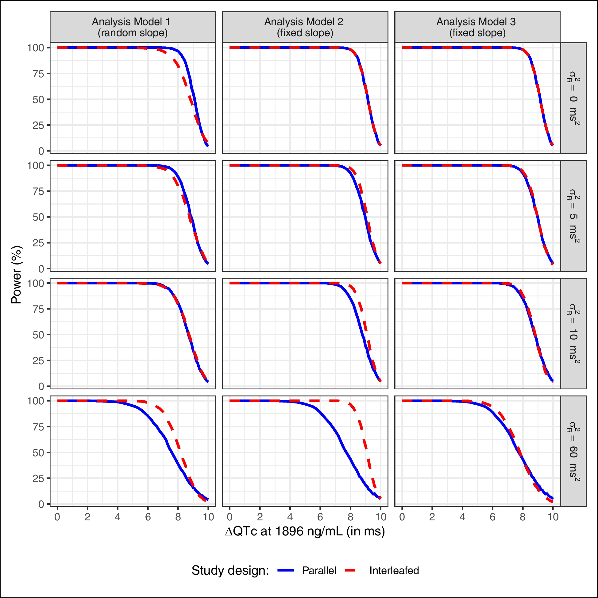
Figure 1 shows that there is no benefit from the interleaved design when \(\sigma ^2_R \le 10\), despite the fact that there can be considerable correlation between observations from different periods. For example, the correlation is 0.5 across all periods and time points when \(\sigma ^2_R = 10\). Figure 2 shows that this does not change when a random slope (\(\sigma ^2_S = 0.00004\)) is added. The considerations in this appendix are an attempt to explain this finding.

In this appendix we provide some additional tables and figures.

Simulation results for parallel ascending group (solid blue line) and interleaved (dashed red line) design with data generation model (6) & random effects models (7) where \(\sigma ^2_U=180 \, ms^2\), \(\sigma ^2_V=10\, ms^2\), \(\sigma ^2_\varepsilon =10\, ms^2\), no random slope (\(\sigma ^2_S=0\, ms^2\)), and with varying values of \(\sigma ^2_R\) in the different rows, when analyzed with Analysis Models 1 (with random slope), left column), and Analysis Models 2 and 3 (without random slope), middle and right columns; values of \(\sigma ^2_R\) differ from those in Fig. 1

Simulation results for parallel ascending group (solid blue line) and interleaved (dashed red line) design with data generation model (6) & random effects models (7) where \(\sigma ^2_U=180 \, ms^2\), \(\sigma ^2_V=10\, ms^2\), \(\sigma ^2_\varepsilon =25\, ms^2\), no random slope (\(\sigma ^2_S=0\, ms^2\)), and with varying values of \(\sigma ^2_R\) in the different rows, when analyzed with Analysis Models 1 (with random slope), left column), and Analysis Models 2 and 3 (without random slope), middle and right columns