
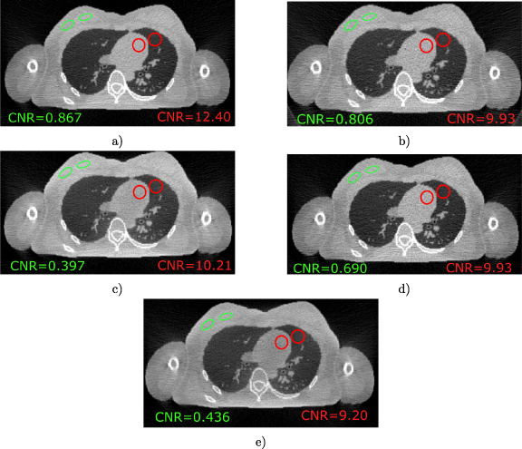
Remember me
Medical imaging is core to modern medicine and drastically improves our ability to better diagnose various illnesses and health problems, enabling better medical treatment. Computed tomography (CT) and radiography are among the medical imaging techniques that have seen a rampant usage over the past decade. A 2022 UNSCEAR report estimates an increase in the amount of annual CT examinations of 86% compared to its previous 2008 report (UNSCEAR 2010, 2022). CT and radiography allow for the visualization of internal tissues of various densities using x-rays. However, the use of ionizing radiation can pose serious health problems, mainly an increased probability of carcinogenesis (UNSCEAR 2010, Sayed et al 2024). Albeit contested (Sacks et al 2016, ANS 2020), the currently most accepted model for estimating health risks from low dose radiation exposure is the linear-no-threshold model (ICRP 2007, UNSCEAR 2010, Boice 2017), meaning any exposure poses a risk of carcinogenesis, with the probability increasing linearly with the dose. It is then always in the best interest of patients to reduce the radiation exposure caused by medical imaging devices while maintaining a sufficient contrast-to-noise ratio (CNR) for an accurate clinical diagnostic. This is especially important in CT, as it is the imaging technique contributing the most to the collective dose worldwide (UNSCEAR 2022).
In x-ray imaging, while low energy x-rays contribute more to contrast, high energy x-rays over 100 keV are required to penetrate large volumes, such as the abdomen (Halliburton et al 2011). To scan larger patients, a tube voltage of 120–140 kVp is typically used at the cost of an increase in radiation dose (Gkanatsios et al 2002, Halliburton et al 2011, Sezdi 2011). Moreover, at these high energies, Compton scattering dominates over photoelectric absorption, which negatively affects the image quality if scattered photons are not removed from the data. The detection of scattered photons blurs the image, decreases its contrast, and introduces various artifacts and CT number inaccuracies, especially in cone-beam CT (CBCT) (Siewerdsen and Jaffray 2001). To remedy this problem, CT scanners use anti-scatter grids (ASGs) placed on the detector array, to reduce the scattered photons contribution to the detector measurements, and thus ultimately to the image at the detriment of the detector’s sensitivity to primary photons. This reduction in sensitivity can be impactful, between 30% and 50% depending on the grid, and is only mitigated by increasing the radiation exposure (Mizuta et al 2012, Rossignol et al 2024b).
Time-of-flight (ToF) scatter rejection has recently been proposed as an alternative to ASGs in CBCT and radiography systems to increase the detector’s sensitivity and therefore reduce the necessary radiation exposure to the patient (Rossignol et al 2020). Instead of using an ASG, this method measures the ToF of x-ray photons from the source to the detector to discriminate between primary photons traveling in a straight line, and scattered photons traveling through a longer path, and thus taking more time to reach the detector. Removing the ASG while keeping an efficient scattering rejection allows for the restoration of the scanner’s sensitivity. A previous simulation study has shown that with a timing resolution of 50 ps full width at half maximum (FWHM) and better, ToF scatter rejection performs as well or even better than an ASG at reducing attenuation values inaccuracy and cup artifacts (Gaudreault et al 2021). As shown in the same study, with the additional benefit of being completely transparent to primary photons, this method can lead to considerable improvement to the CNR, even at 50 ps FWHM timing resolution. Previous studies on ToF scatter rejection (Rossignol et al 2020, Gaudreault et al 2021) resorted to simulations using a very simple phantom composed of a water container with a few cylindrical inserts.
This method is designed specifically for photon counting CT (PCCT) and can benefit from all of its advantages such as the elimination of electric noise, energy weighting, improved spectral CT (Willemink et al 2018, Rajendran et al 2022). However, contrary to all current clinical PCCT scanners that use a direct semiconductor detector, ToF scatter rejection requires a scintillation-based detector to achieve a better timing resolution (Greffier et al 2025). A scintillation-based detector comes with additional challenges in regards to reaching a high enough count rate, but recent studies support its feasibility (van der Sar et al 2021) and a scanner reached a count rate of 8 MHz (Sato et al 2025).
This paper aims at providing additional data on the performance of ToF scatter rejection using a more realistic phantom. Moreover, with the goal of reducing health risks induced by ionizing radiation, it focuses on characterizing the performance in terms of dose reduction to image quality.
First, the different simulation setups will be presented, followed by a description of the virtual ASG used to replicate an ASG in simulation without heavy memory requirement. Then, the comparison metric chosen is explained along with the necessary adjustments that had to be made to reduce simulation-to-simulation variance without hundreds of heavy and time consuming simulations of CT scans.
To characterize the dose reduction with ToF scatter rejection, this paper compares the radiation exposure needed to achieve a set image quality quantified in terms of the CNR for different hardware-based scatter rejection techniques.
Ideally, image quality should be measured throughout every simulation, and then the radiation exposure needed for each method could be compared where the image quality meets. Moreover, due to the stochastic nature of x-ray imaging, the process should be repeated to reduce variance. However, since CT simulations are very time-consuming, an alternative method was used. Only one full scan was simulated for each scatter rejection method, and the resulting data was used to generate all the other needed images of lower dose and quality with a statistical adjustment to include noise as if a new simulation had been carried out.
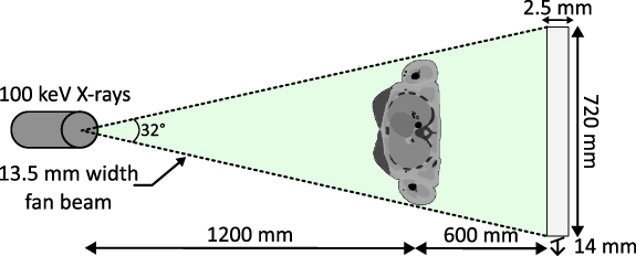
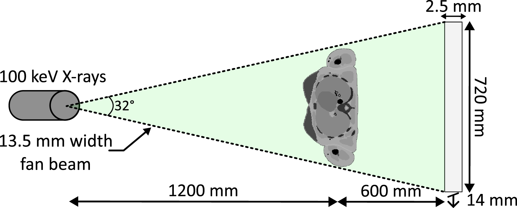
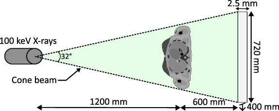
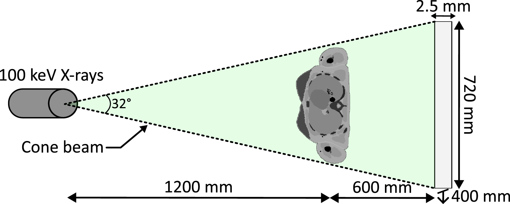
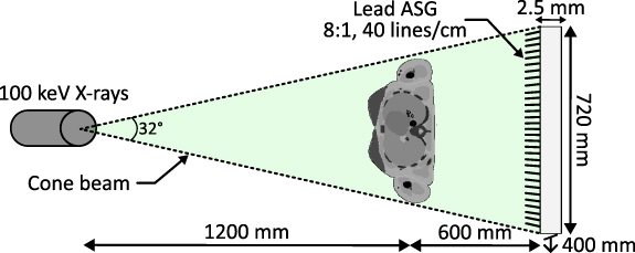
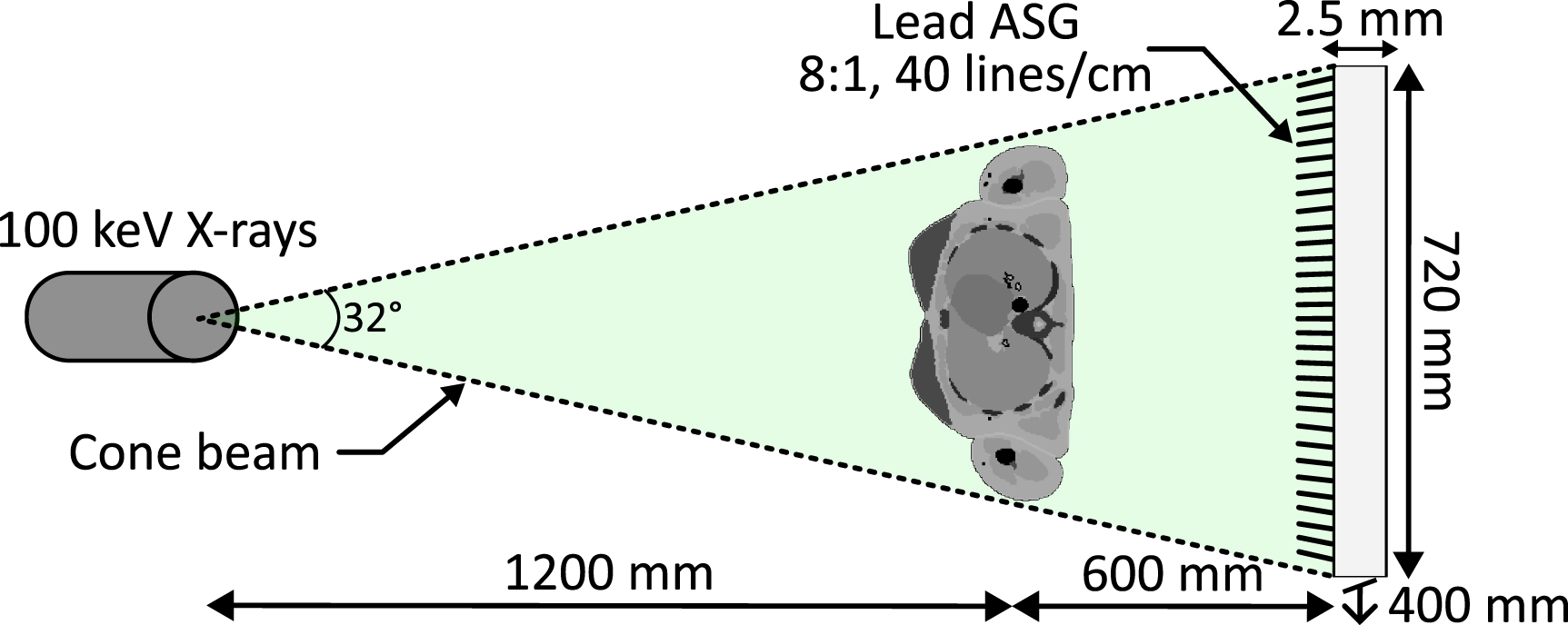
2.1. Simulation setupsThe Monte Carlo simulation software GEANT4 Application for Tomographic Emission (GATE) (Agostinelli et al 2003, Jan et al 2011, Sarrut et al 2014) was used to simulate and assess performance of an upper body CT scan with three different scanner types: a step-and-shoot fan-beam multi-slice CT (MSCT), a CBCT with an ASG, and a CBCT with ToF scatter rejection. In order to have sufficient penetration while keeping the energy factor constant, all three simulations used a monochromatic x-ray source set at 100 keV which differ from the typical bremsstrahlung spectrum. This was done to reduce the number of variables and enable an easier analysis of the data for this early method characterization. This change also increases the number of scattered photons, especially in the forward direction. For all experiments, the source is placed 120 cm in front of the phantom, which is located 60 cm in front of the detector (figures 1–3). A flat monolithic block of LYSO of 720 × 400 × 2.5 mm3 was used as a detector for both cone-beam scanners, while a 720 × 14 × 2.5 mm3 detector of the same material was used for the fan-beam scanner. The flat panel is pixelated in post-processing with a pixel size of 2 × 2 × 2.5 mm3. Pixelating the detector in post-processing, as opposed to directly using a pixelated LYSO detector in GATE, was found to decrease the simulation time. A whole-body voxel phantom of a reference adult female, developed and published by the ICRP, with a pixel resolution of 1.775 × 1.775 × 4.84 mm3 is imaged (ICRP 2009).
Figure 1. Step-and-shoot fan-beam multi-slice CT simulation setup.
Download figure:
Standard image High-resolution imageFigure 2. Cone-beam CT with ToF simulation geometry and configuration.
Download figure:
Standard image High-resolution imageFigure 3. Cone-beam CT with anti-scatter grid simulation geometry and configuration.
Download figure:
Standard image High-resolution imageIn this study, the scintillation process in the LYSO was not simulated, as it significantly increases the processing time. Instead, the GATE simulations directly output the point of interaction, the energy, and the ToF of each x-ray photon detected in the LYSO for image reconstruction. Additionally, the detector has a photon energy threshold of 20 keV, below which the detection is discarded. From the GATE data, a 360 × 360 × 200 pixels sinogram was generated, owing to the 360 projections acquired around the phantom.
2.1.1. Step-and-shoot fan-beam MSCTThe first simulation used step-and-shoot MSCT with a constant beam thickness of 13.5 mm, sliding along the height of the phantom. The image is reconstructed with a filtered back projection algorithm using the ASTRA toolbox 2.1 Python library (van Aarle et al 2016) with a final voxel size of 1 mm3. This image serves as a reference for comparison with other images.
2.1.2. CBCT with ToF scatter rejectionThe second CT scan was simulated with the CBCT configuration depicted in figure 2 for which the scattered photons are filtered out with a simple time threshold using their ToF with a normally distributed timing jitter of 10, 50, 100, 200 ps FWHM to simulate the respective uncertainties of timing measurements of a real system. These uncertainties include the pulsed x-ray width and the detector’s jitter.
Since the measured ToF of ballistic and scattered photons overlap due to timing uncertainties, the time threshold for the discrimination between scattered and ballistic photons was set slightly higher to 11, 54, 114, 222 ps respectively to limit the loss of primary photons while maintaining sufficient efficiency (Rossignol et al 2024b). A CT image with ToF scatter rejection is reconstructed for each timing jitter with an FDK (Feldkamp et al 1984) algorithm implemented in the ASTRA toolbox 2.1 Python library (van Aarle et al 2016) with a final voxel size of 1 mm3. In total, four images with varying quality resulting from different timing jitters are generated to observe their effect in CT. Lastly, an additional image with no time filtering, thus a regular photon counting image without an ASG, is also produced for comparison.
2.1.3. CBCT with ASGThe third simulated scanner is identical to the previous setup, with the addition of a focused ASG made of strips spanning the entire surface of the detector. Also, a continuous 100 keV source is used instead of the pulsed x-ray source.
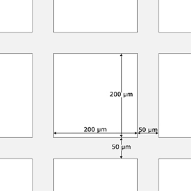
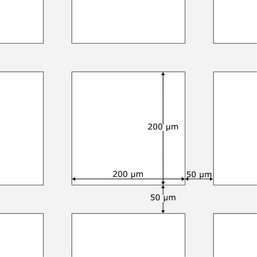
The ASG (figure 4) has focused square holes with a septal thickness (grid thickness) of 50 µm, an interspace (hole diameter) of 200 µm and a height of 1.6 mm (8:1 ratio), resulting in a grid frequency of 40 lines cm−1. This ASG is chosen to enable comparison with a real ASG used in a study on the effect of ASGs in CBCT (Schafer et al 2012). Unfortunately, due to memory and complexity limitations of GATE’s volume modeling system, such a dense grid could not be modeled without considerable slowdowns. For this reason, GATE’s code was instead modified to incorporate a virtual ASG as a GATE Actor. The grid surface is modeled as a group of mathematical 2D planes in 3D space, and the particle entering the grid’s boundary is modeled as a straight line. If the photon’s trajectory intersects with one of the grid planes, the photon is removed, otherwise, it continues its trajectory. With this approach, the virtual grid absorbs every photon entering in contact with it, meaning photons cannot scatter in the grid. Therefore, its scattered transmission ( ) is very close to 0, making it more efficient than a real ASG, which for an 8:1 ratio should have a
  around 0.17 (Mizuta et al 2012). In the future, a more realistic ASG model could be implemented to better represent the real ASG’s behavior.
Figure 4. Schematic of a section of the ASG model used in this study.
Download figure:
Standard image High-resolution image 2.2. Dose evaluationThe dose measurements are performed in two ways. First, due to all three scans irradiating the exact same part of the phantom, the total amount of photons emitted from the source per unit area can be used to compare radiation exposure between the different methods.
Second, it is also possible to obtain more precise values to potentially enable comparison to other literature in the future. During the simulations, the DoseActor and DoseByRegion functions included in the GATE dosimetry module estimate the deposited energy in every phantom voxel, thus enabling estimation in each individual tissue or organ (Sarrut et al 2014). The effective dose can then be compared with the reconstructed image and its CNR. The effective dose E, expressed in Sieverts (Sv) is calculated from the following equations:


where HT the equivalent dose measured in a specific tissue, calculated from the radiation weighting factor wR for radiation type R and the absorbed dose  , in tissue T by radiation type R. From the equivalent dose, the effective dose E can be calculated by using the the tissue weighting factor wT as published by the ICRP (ICRP 2007). The absorbed dose describes the energy deposited per unit of mass and is directly given by GATE. Only x-rays, which have a given radiation weighting factor of 1 (ICRP 2007), are considered in this case. Thus, the equivalent dose is equal to the absorbed dose.
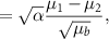
Simulations of a torso slice for each scan are generated with about an equal density of emitted photons from the source. Therefore, the images were generated with the same radiation exposure to the body but differed in their image quality. In this study, the image quality is quantified with the CNR calculated as follows (Kawashima et al 2018):

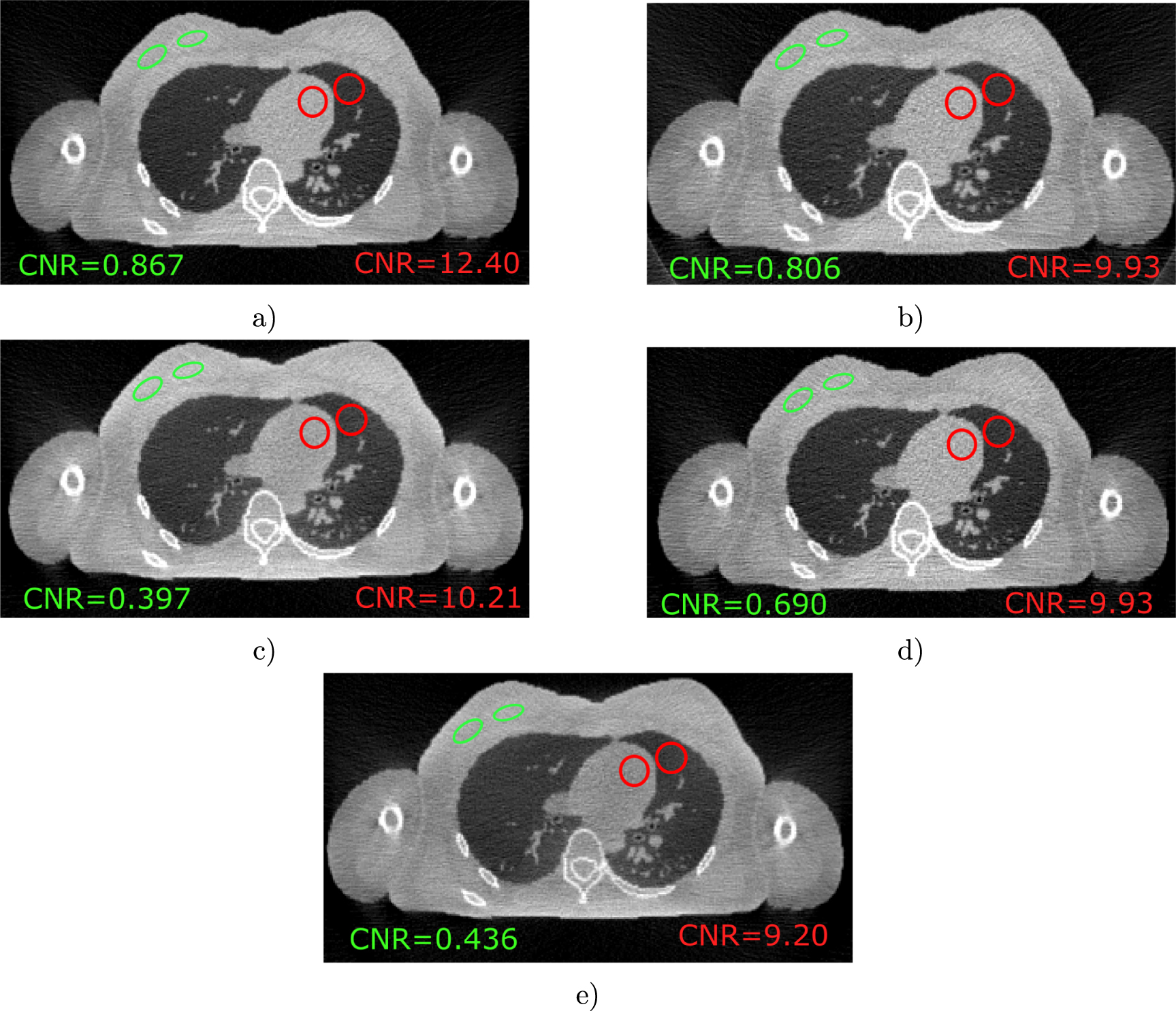
where µ1 and µ2 are the mean pixel value of a region of interest composed of the higher density region (1) and its surrounding lower density region (2). σb is the background noise taken as the standard deviation of a circle region in the lungs. Two regions of interests (ROIs) are measured : the heart-lung region, representing high contrast conditions, and the breast tissue region between the higher density mammary gland and its surrounding lower density adipose tissue, representing low contrast conditions. The heart-lung and breast tissue ROIs, are shown in figure 5 as red and green circles respectively.
Figure 5. Axial slice through the torso of the AF ICRP phantom for (a) the full 10 ps CBCT TOF, (b) the full CBCT with ASG, (c) the full 200 ps CBCT TOF, (d) the CNR adjusted 10 ps CBCT ToF (with 63% of photon counts), and (e) the full slice without scatter rejection. Red and green circles correspond to the ROIs used in calculating the CNR.
Download figure:
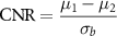
Standard image High-resolution imageFor what follows, it is important to note that for a CT scan, the CNR should be proportional to the square root of the exposure. This is because a CT scan inherently follows a Poisson process for which the variance ( is equal to the expected value (µ), meaning:

Increasing or decreasing the number of photons by a factor α directly scales the mean of each pixel such that  , therefore

and thus,

This property can be used directly to calculate the CNR analytically at any exposure and therefore derive the dose reduction for a fixed CNR. However, as to not solely rely on this presumed property, the following data driven approach is also used and then compared with the analytical approach.
As mentioned in the introduction of the methods section, to avoid having to simulate hundreds of CT scans, the original data for each simulation was used to generate a series of images with lower radiation exposure, thus leading to a lower CNR. To do so, an approximation using a statistical approach was applied on the generated sinograms to estimate the image data at a lower photon count. To reduce simulation-to-simulation variance, 50 images are reconstructed for each exposure factor  upon which the CNRs are calculated and averaged. The radiation exposure is then compared at a point where all CNRs are equal.
More specifically, the photon count is reduced by multiplying the sinogram’s pixel values by the factor α. Then, for each pixel, statistical noise is added by taking 50 new random values from a Poisson distribution with the mean λ of the distribution equal to the pixel value. The 50 new unique sinograms are reconstructed, and the CNR is calculated for each and then averaged. Given that for a Poisson distribution the expected value is also equal to the variance, if the original images did not contain any noise, the resulting CNRs should follow equation (5). However, since the original images do contain Poisson noise already, the effect on the CNR is slightly different and needs to be adjusted. First there is the multiplication by α to adjust the mean count, having no effect on the CNR since the noise is affected in the same way:
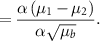
This is followed by the addition of the Poisson noise from the random sampling, which is done by adding both variances together :
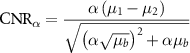
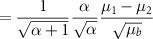
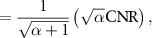
and thus

One can see that the statistical noise of the original images contributes a factor of  . To account for the noise, the CNRs were simply adjusted by multiplying by the inverse factor to compensate the error. The derivation of equation (7) does assume some Poisson statistics. Therefore, to validate the procedure, the resulting CNR should coincide with the expected CNR proportionality to the square root of the photon count (equation (5)).
Figures 5(a)–(c) show the original reconstructed images prior to CNR calibration for different scans or timing, which can be visually compared with the image without any scatter rejection or correction applied shown in figure 5(e). Each image is presented with the same window levels and contrast to enable a fair visual comparison. These images were generated with the same number of photons going through the patient and therefore for the same radiation exposure. The reconstructed images with CNR value adjusted using the data driven approach are shown in the bottom right. Figure 5(d) shows the 10 ps CBCT image after it has been adjusted to have the same CNR as in figure 5(b).
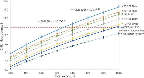
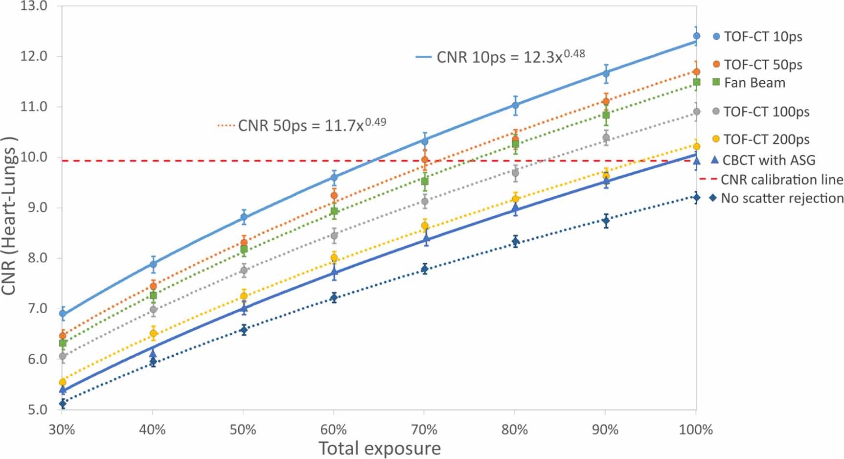
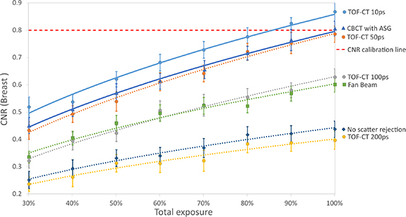
In figures 6 and 7, the points of intersection between the horizontal dotted red line and the CNR curves represent the number of photons expressed as a percent exposure required by each respective scanning method to achieve the same image quality quantified as a CNR (a CNR of 9.93 is considered for the heart ROI and 0.8 for the breast ROI). Thus, the dose reduction compared to the CBCT with ASG scan can be directly inferred from those intersection points.
Figure 6. CNR values of the heart ROI based on the photon count expressed as a percent exposure used to reconstruct the image with a power function fit applied. The dotted red line represents the CNR for CBCT with ASG at 100% photon count. The error bars represent the CNR’s 95% confidence interval from 50 reconstructed CT images.
Download figure:
Standard image High-resolution imageFigure 7. CNR values of the breast ROI based on the photon count expressed as a percent exposure used to reconstruct the image with a power function fit applied. The dotted red line represents the CNR for CBCT with ASG at 100% photon count. The error bars represent the CNR’s 95% confidence interval from 50 reconstructed CT images.
Download figure:
Standard image High-resolution imageThe CNR values in table 1 are taken directly from the original full images. Following figure 6, the dose reduction shown represents the reduction in photon count required to achieve the same CNR as the CBCT with ASG, taken from the intersection point between the calibration line and power function fitting of each scan.
Table 1. Dose reduction after CNR calibration for the heart-lung ROI, relative to CBCT with ASG.
SimulationCNR at 100% photon (α = 1)Dose reduction (at )CB TOF 10 ps12.435%CB TOF 50 ps11.728%CB TOF 100 ps10.915%CB TOF 200 ps10.25%Fan beam11.525%CB with ASG9.90%4.1. Interpretation
For both ROIs, ToF scatter filtering on CBCT at 10 ps FWHM (figure 5(a)) shows visible improvements in contrast over the ASG method (figure 5(b)) at equal photon counts. The image also looks slightly sharper around the bones and in the lungs. The attenuated CBCT with ToF at 10 ps FWHM (figure 5(d)), calibrated to have a CNR equal to the ASG’s image, visually shows a reduction in contrast and an increase in statistical noise when compared to its original (figure 5(a)). It is overall much closer to the ASG’s image than the original 10 ps ToF image. However, it is important to note that this image contains more noise than it should since its CNR follows equation (7), before the adjustment by a factor of  .
.
Figures 5(c) and (e), unlike the others, are polluted by a significant amount of scattered photon data due to the worse timing resolution. Because of this, the images look less noisy but also washed out and the contrast is reduced. Visual artifacts around high density areas like the bones are much more present and the centre of the image is darker, representative of a cupping artifact.
The visual improvement is validated by the CNR values measured between the lungs and the heart and showcased in figure 6 and table 1. Interestingly, in the case of the heart ROI, ToF scatter rejection at 10 and 50 ps FWHM even gives a +10% and +3% improvement in dose reduction over the fan beam image without ASG. For this region, the ASG only brings small improvements when compared with the image without any scatter correction. This is not surprising as the use of a grid can often result in very minimal or even a loss of CNR at equal dose due to the loss in sensitivity, with the advantage of increasing CT number accuracy (Schafer et al 2012). However, in the case of the ROI between breast tissues circled in green, figure 7 and table 2 show the ASG performs better than ToF at all resolutions but 10 ps FWHM. This difference in results between both ROIs can be explained by the much lower contrast between the breast tissues compared to the heart-lung region. Therefore, the relative impact of scatter on the region is stronger, and only 10–50 ps ToF is able to remove enough scatter to restore the CNR. Moreover, this study uses an ideal ASG which does not let any scatter through. When matching our grid of a 8:1 ratio to a comparison table of various ASGs, we could expect a real grid to have a scatter transmission  between 13%–17% (Mizuta et al 2012). Additionally, the poor results at 100–200 ps FWHM ToF in the breast region could be due to the fact that the current time threshold based method used to discriminate scattered photons from primaries is independent of the position. The same threshold is used for a detector pixel in the center than a pixel on the edge of the detector, which could lead to poorly optimized threshold values in some region of the image due to the variation in scattered photon’s ToF across the detector area. It seems to be especially the case for 200 ps Tof in the breast region which obtains worse results than when not using any scatter correction at all. This highlights the need for more advanced scatter rejection algorithms than a naive static time threshold. This idea is explored in other work using a deconvolution method (Rossignol et al 2024a).
Table 2. Dose reduction after CNR calibration for the breast ROI, relative to CBCT with ASG (Negative values indicate an increase in dose).
SimulationCNR at 100% photon (α = 1)Dose reduction (at )CB TOF 10 ps0.86715%CB TOF 50 ps0.785−5%CB TOF 100 ps0.628−174%CB TOF 200 ps0.337−384%Fan beam0.600−73%CB with ASG0.8060%4.2. Virtual ASG
In this simulation study, the ASG (figure 4), unlike every other object in the set-up, is not modeled as a physical GATE volume, meaning GATE is not calculating every particle movement and interaction like scattering within the grid. Instead, the grid is modeled as a series of planes forming the surface of the ASG, and every particle whose trajectory intersect with one of those planes is deleted from the simulation. Whereas a real grid would still scatter photons, increasing its blocking efficiency and inducing a small amount of scatter noise, the virtual ASG has a scattered photons’ transmission close to 0, thus improving the results of the CBCT with ASG.
This model was chosen for its simplicity and creates a slight bias favoring CBCT with ASG. Since this study aims at quantifying the improvement the ToF scatter rejection method can have on the ASG method, it is important to avoid favoring ToF-CT in the approximations.
It is interesting to note that for an almost perfect timing resolution (10 ps and lower as shown in Gaudreault et al (2021)) and a known perfect grid model (i.e. all scattered photons are filtered out), the only difference between the two methods is the considerable attenuation of primary photons by the ASG. This property of ASGs is inversely characterized by the primaries’ transmission,  . In this case, it is possible to calculate the exact reduction in radiation exposure between the ToF and the ASG method by calculating the area of the detector covered by the grid:
Due to the idealistic nature of the grid, we can assume that the grid’s transmission of primary photons is equivalent to the effective area of its holes to the total area of the detector as seen from the source’s position:

where  is the primary photon transmission across the ASG, i.e. the ratio between the number of primary photons after and before the grid. The effective area is then calculated using the ratio between the area of a hole and the area of a whole unit section, which includes the grid solid segments and the hole as follows:
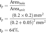
With such a grid, only 64% of the primary photons would go through and contribute to the detected signal. Therefore, with a perfect ToF CT scanner, only 64% of the exposition would be needed to acquire the same primary signal, leading to a dose reduction of  . This theoretical value is very close to the simulated value of 35% with 10 ps ToF scatter rejection in the heart ROI.
When comparing the results from the heart region, the trends of the results for different timing resolutions is closely matched by a similar simulation study, conducted by Gaudreault et al (2021), on the impact of ToF scatter rejection on the CNR. However, the CNR improvements between a CBCT with ASG and a CBCT using ToF scatter rejection differ at higher timing resolutions (10 ps and 50 ps FWHM). This discrepancy can partially be explained by the higher grid frequency used in Gaudreault et al leading to an effective detection area of 53% as opposed to 64% in the present study. Moreover, the present study simulates a scan of a complex adult female phantom, while in Gaudreault et al the phantom is a simple water-filled cylinder with two bone inserts. The difference in composition, complexity, and thickness can heavily impact ToF scatter rejection results, especially since the current rejection method used is a simple static time threshold. Past studies had not looked at low contrast soft tissue regions, thus, the results cannot be compared as of yet.
4.4. Other considerationsAs expected, the power fits applied to the CNR values in figure 6, in every case, resulted in an equation of the form:

where k is an amplification factor proper to each curve, and α is the relative number of photons used to reconstruct the images. Since the CNR must be directly proportional to the square root of the photon count, the power value resulting from the fit, being approximately 0.5 for all curves, validates the method used for CNR calibration.
While it has already been shown that ToF scatter discrimination can reduce scatter noise to boost the image quality in CBCT images at equivalent dose (Gaudreault et al 2021), this simulation study shows the method’s potential in reducing the radiation exposure at equivalent image quality for a realistic phantom. Using a simple time threshold method, simulated data for ToF CBCT with 10–50 ps tim
Comments (0)