Pulse sequence design and implementation

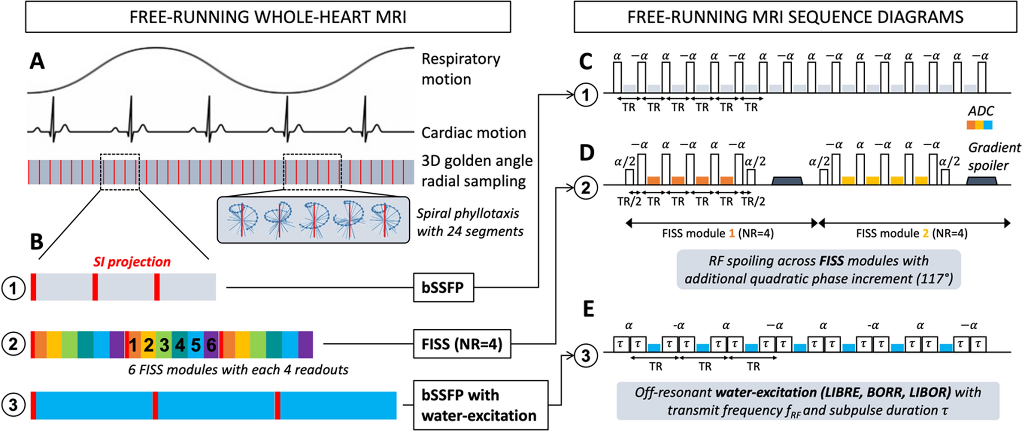
Data are continuously acquired in free-running MRI, irrespective of cardiac and respiratory motion (Fig. 1A). Different methods for fat signal suppression were evaluated (Fig. 1B), a standard bSSFP acquisition (Fig. 1C), a FISS acquisition (Fig. 1D), and three different types of off-resonant water excitation RF pulses integrated in a bSSFP acquisition (Fig. 1E). Both the free-running bSSFP and FISS sequences use nonselective rectangular RF pulses with a duration of 0.3 ms.

Fig. 1

Schematic overview of the free-running MRI sequences. Data acquisition is performed continuously, irrespective of cardiac and respiratory motion (A). Different acquisitions for fat signal suppression were performed (B); a free-running bSSFP sequence with standard rectangular excitation pulses (C), a FISS sequence with standard rectangular excitation pulses (D), a bSSFP sequence with BORR, LIBRE, and LIBOR water excitation pulses (E). Numerical simulations were performed to tune the RF pulse parameters, which were experimentally verified

The FISS sequence is an interrupted bSSFP sequence, dividing it into FISS modules, as described in [35]. A FISS module starts with a ramp-down pulse (α/2) and ends with a magnetization restoration pulse (α/2). Four readouts were acquired per FISS module (NR = 4), a 117° quadratic RF spoiling was applied across FISS modules, and gradient spoilers were inserted after each FISS module. Note that all described implementations are embedded within the same MRI sequence.

As described previously, the LIBOR [20], BORR [20, 25], and LIBRE [27] RF pulses follow a binomial 1-1 pattern, consisting of two subpulses with variable subpulse duration τ. For all three pulses, shortening the RF pulse duration requires an increase in the off-resonance frequency. As a result, the RF power needs to increase to excite the water magnetization to the desired rotation angle. The main differences between these three water excitation pulses are the phase offset of the second subpulse Δφ2 and the required RF power, which changes their SAR signature.

More specifically, the BORR pulse is defined by a fixed 180° phase modulation on the second subpulse [25, 26]. The LIBRE pulse has a phase offset that depends on the subpulse duration and the RF pulse frequency Δφ2 = 2πfRFτ [27]. To reduce RF power, the LIBOR pulse is defined by an RF pulse frequency that is half that of the LIBRE pulse, after which the phase offset is adjusted to achieve fat signal suppression [20]. So far, only the LIBRE pulse has been used at 1.5 T [19], for which the subpulse duration was set to 1.3 ms, leading to a total RF duration of 2.7 ms. Therefore, in the current study, the duration of all pulses was standardized to this value for a fair comparison.

To determine the LIBOR phase offset, numerical simulations of the Bloch equations were performed, which was subsequently verified in phantom experiments. The transverse magnetization Mxy as a function of the phase offset and off-resonance after a single LIBOR RF excitation was simulated using an RF excitation angle of 50° and an off-resonance frequency of 270 Hz. This frequency is half that of the 540 Hz off-resonance frequency of the LIBRE pulse at 1.5 T, which was found based on an iterative simulation. The off-resonance was varied between − 800 Hz and 800 Hz in steps of 10 Hz, and the phase offset was varied between 0° and 360° in steps of 10°. The phase offset corresponding to the widest signal suppression band around fat (− 220 Hz), defined as 10% of the maximum observed transverse magnetization (Mxy), was selected for subsequent measurements. All simulations were performed in MATLAB 2021 (The MathWorks, Natick, MA, USA). The code for this simulation can be found on GitHub.

Another set of simulations was performed to calculate the RF power adjustment for all RF pulses. This was done by simulating the RF pulse response, meaning the transverse magnetization Mxy as a function of off-resonance following a single RF pulse excitation using either a LIBOR, BORR, LIBRE, or a single nonselective rectangular pulse. This RF response was then used to calculate the RF power adjustment to ensure a 50° rotation of the water magnetization, referred to as the nominal RF excitation angle. The off-resonance was varied between − 800 Hz and 800 Hz in steps of 10 Hz; the off-resonance frequency of LIBRE was set to 540 Hz, that of LIBOR to 270 Hz, BORR to 500 Hz, and the standard rectangular pulses to 0 Hz. The BORR transmit frequency of 500 Hz was chosen based on its optimal signal suppression at – 220 Hz. The results of these simulations informed on RF power increases for subsequent MRI experiments, which were achieved by increasing the RF excitation angle in the user interface of the MRI sequence. The RF waveforms corresponding to each of the RF pulses were plotted for comparison.

Numerical simulations of free-running FISS and bSSFP sequences with and without off-resonant water excitation pulses

The steady-state transverse magnetization Mxy was simulated as a function of RF excitation angle and off-resonance for a bSSFP and a FISS sequence with nonselective RF excitation pulses, as well as a bSSFP sequence with LIBOR, LIBRE, and BORR RF excitation pulses. The RF properties found in the previous section were used (Table 1). RF excitation angles were varied around their previously determined optimal RF excitation angle by − 20° to + 20° in steps of 5°. The off-resonance was varied between − 800 Hz and 800 Hz in steps of 10 Hz. The repetition time (TR) was set to the minimum possible at the MRI scanner and was 2.47 ms for FISS and bSSFP and 4.9 ms for the bSSFP sequence with integrated LIBRE, BORR, and LIBOR pulses. A T1 of 1390 ms and T2 of 300 ms was used to reflect the relaxation times of blood at 1.5 T. To ensure a magnetization steady state, 1000 RF excitations were simulated. In the case of FISS, perfect RF and gradient spoiling were simulated by nulling the Mxy after each FISS module. The result of these simulations provides a comparison of water excitation efficiency, i.e., the required increase in power deposit relative to on-resonant pulses, fat signal suppression, and corresponding suppression bandwidths.

Table 1 MRI acquisition parameters and RF pulse propertiesValidation of fat signal suppression in a fat phantom

To validate fat signal suppression, MRI experiments were performed using a 3D radial free-running bSSFP MRI sequence with different off-resonant water excitation methods on a 1.5 T clinical MRI scanner (MAGNETOM Sola, Siemens Healthcare, Erlangen, Germany). Each experimental setup was repeated three times over three separate days. The fat phantom contained vials with different fat percentages, ranging from 0 to 100% of water and peanut oil mixtures, as described in [36].

The study included two independent sets of experiments. First, the RF excitation frequency offset, RF excitation angle, and LIBOR phase offset were varied systematically to compute water and fat contrast in the resulting images. The initial parameters were guided by the results of the numerical simulations. In the second experiment, the effectiveness of fat signal suppression for every pulse was compared using the RF parameters from the first phantom experiment. The FISS sequence was also included in this comparison, with its parameters taken from our prior work [22]. Note that the exact same FISS sequence was used in the current study, which allows switching to bSSFP and switching between RF excitation pulses from the user interface.

To test the effect of RF excitation frequency offset on the measured signal, the RF excitation angle was kept constant. For BORR, with a fixed RF excitation angle of 141°, the frequency was varied from 400 to 600 Hz in steps of 20 Hz. For LIBRE, with an RF excitation angle of 124°, the same frequency range was used. For LIBOR, with an RF excitation angle of 78° and a phase offset of 285°, the frequency was varied from 250 to 340 Hz in 10 Hz increments.

To test the effect of RF excitation angle on the measured signal, the RF excitation frequency was held constant. For BORR, the RF excitation angles were varied in 10° increments from 90° to 180°, while keeping the frequency fixed to 600 Hz, using a frequency offset of 600 Hz. For LIBRE, the RF excitation angles were varied from 50° to 180° in steps of 10°, using a frequency of 500 Hz. For LIBOR, with a frequency offset of 270 Hz and a phase offset of 285°, RF excitation angles ranged from 50° to 100° in steps of 5°.

Finally, to determine the effect of the LIBOR phase offset on the water-fat contrast, a phase offset sweep from 250° to 340°, with steps of 10°, was performed. The LIBOR pulse using frequency was 270 Hz with an RF excitation angle of 78°.

Further acquisition parameters were constant and included: a field of view (FOV) of 220 × 220 × 220 mm3, matrix size of 112 × 112 × 112, a  (2.0 mm)3 isotropic resolution, a 992 Hz/pixel bandwidth (BW). The radial trajectory used 24 lines per interleaf with 246 interleaves for a total of 5904 radial readouts, efficiently sampling the entire 3D k-space to ensure comprehensive volumetric data acquisition. The echo time (TE) and repetition time (TR) varied per experiments (Table 1).

The phantom results were used to decide on the RF parameters for the whole-heart MRI experiments (Table 1). This final protocol was tested in a phantom with an increased number of radial readouts (24 × 1877). A FISS acquisition was added for comparison.

Contrast-free 5D whole-heart free-running MRI in volunteers

Five healthy volunteers (n = 5; 4 females; 27.4 ± 7.5 years old; height 168.8 ± 7.8 cm; weight 64.4 ± 10.9 kg) participated in this study, who provided written and informed consent approved by our local ethical review board.

The volunteer’s protocol was based on the ECG-triggered non-interrupted 3D radial free-running bSSFP sequence, as used in the comparison setup for the phantom experiment (Table 1). The data were acquired on a 1.5 T clinical MRI scanner (MAGNETOM Sola, Siemens Healthcare, Erlangen, Germany) with four fat suppression methods (FISS, BORR, LIBRE, and LIBOR), along with a bSSFP sequence without any fat signal suppression. This comparison followed a similar setup described in a previous study by Masala et al. [19], where a 32-channel spine coil and an 18-channel chest coil were used during the free-breathing acquisition. The radial readouts were arranged in interleaves based on a spiral phyllotaxis pattern, with successive interleaves rotated about the z-axis by the golden angle, and the first readout in each interleave oriented in the superior-inferior (SI) direction for subsequent physiological motion extraction and binning into cardiac and respiratory phases.

Because of differences in RF pulse duration, the TR was 2.47 ms for bSSFP and FISS, and 4.9 ms for LIBRE, LIBOR, and BORR. The total number of acquired radial lines was constant using a spiral phyllotaxis trajectory consisting of 1877 spirals, with each 24 k-space segments. The resulting acquisition time for each sequence was constant for all volunteers, independent of their respiratory pattern and heart rates, with 3 min and 41 s for BORR, LIBRE, and LIBOR, 2 min and 55 s for FISS, and 1 min and 51 s for the bSSFP sequence without fat suppression.

5D whole-heart motion resolved volunteer image reconstruction

The volunteer data were reconstructed using an in-house MATLAB code, following the free-running framework described by Di Sopra et al. [37]. Two separate reconstructions were performed: first, a reconstruction without motion correction to maintain the noise properties for quantitative analysis, specifically for SNR and contrast-to-noise ratio (CNR) comparisons. This reconstruction used radially sampled k-space data with coil sensitivity combination, implemented using the gpuNUFFT library. The coil sensitivity maps were estimated using ESPIRiT from auto-calibrated signal (ACS) data embedded within the free-running acquisition, following the reconstruction pipeline described by Di Sopra et al. [37]. The offline pipeline includes density compensation, NUFFT-based reconstruction without motion correction, and iterative SENSE reconstruction. Second, a compressed sensing reconstruction was carried out to generate 5D cardiac and respiratory motion-resolved images. This was achieved using the alternating direction method of multipliers (ADMM) algorithm [37, 38].

To enhance the quality of image reconstruction and improve local low-rank (LLR) representations, several regularization techniques are possible, including total variation in the cardiac (TVt), respiratory (TVr), and spatial (TVs) dimensions, as well as local low-rank constraints on cardiac (LRtWeight) and respiratory dimensions (LRrWeight). The regularization weights were optimized through a grid search to achieve the best compromise between preserving image detail and minimizing noise. The selected weights were set as follows: TVsWeight = 0, TVtWeight = 0.01, TVrWeight = 0.01, LRtWeight = 0.05, and LRrWeight = 0.05. This combination effectively suppressed artifacts and noise while maintaining both the spatial and temporal resolution of the reconstructed images, which were then used for qualitative assessments of cardiac and respiratory motion.

The motion-resolved reconstruction included four respiratory phases and 25 cardiac phases, allowing detailed visualization of both cardiac and respiratory motion throughout the imaging volume.

The reconstruction time for each dataset was approximately 3 h, executed using MATLAB R2022b on an Ubuntu 22.04.3 workstation equipped with two 32-core CPUs (AMD Ryzen Threadripper 2990WX, Santa Clara, CA), 128 GB of RAM, and an NVIDIA GeForce RTX 2080 Ti (Nvidia, Santa Clara, CA).

Data analysis

Phantom MRI data were reconstructed at the scanner using the vendor-provided pipeline, including predefined coil combinations and gridding optimized for radial trajectories. These phantom images were processed as a single phase without binning or temporal regularization. Because the inline reconstruction does not support motion-resolved or compressed sensing methods, the offline reconstructions were performed in MATLAB as described by Di Sopra et al. [37]. The SNR was calculated in selected regions of interest (ROIs) on the same fat fraction vial in each acquisition, ensuring consistent relative positioning across all images. For SNR measurements, the noise standard deviation (SD) was measured in background regions carefully selected to be free from structured artifacts, residual aliasing, or streaking. Multiple noise ROIs were assessed across different acquisitions to verify consistency in background noise distribution. While coil sensitivity estimation in signal-free regions has inherent limitations, this approach provides a reasonable approximation of system noise when regions are appropriately chosen. For signal measurements, ROIs were placed well within homogeneous regions of the phantom and tissues, avoiding boundaries where potential Gibbs ringing or partial volume effects could influence measurements. SNR was then calculated as the ratio of the mean signal within the ROI to the SD of the background noise. All measurements were conducted using ImageJ software (National Institutes of Health, Wisconsin University, Bethesda, MD), with uniform brightness and contrast settings applied to maintain consistency across images. For CNR calculations, the difference in SNR between two distinct ROIs was computed.

In the volunteer studies, SNR and CNR calculations were based on 3D reconstruction without motion correction to retain original noise properties. SNR was measured using ROIs drawn in the septal myocardium, left ventricular blood pool, chest fat, right lung, and background, in the axial view, being visually chosen for ROI placement. The CNRs were calculated by subtracting the blood pool SNR from the chest fat SNR (CNRBlood-Fat) and the myocardium SNR (CNRBlood-Myocardium). For the 5D motion-resolved images, only qualitative assessments were performed, as the compressed sensing (CS) reconstruction altered the noise characteristics, rendering standard SNR and CNR measurements unsuitable. Since these analyses focused on objective, quantitative measurements rather than subjective evaluations, no additional blinding to pulse sequences was deemed necessary.

For both phantom and volunteer studies, the specific absorption rate (SAR) values, representing RF energy absorption levels, were retrieved from the DICOM files. These values were compared between different acquisitions to evaluate the relative RF energy absorption levels.

Statistical analysis

All results are reported as means ± standard deviations. A one-way analysis of variance (ANOVA) was conducted to evaluate differences in SNR and CNR between the pulse sequences, with statistical significance set at p < 0.05. If significant differences were detected, Tukey’s Honestly Significant Difference (HSD) test was applied as a post-hoc analysis to identify pairwise differences while controlling for Type I errors.

SAR values were measured for each sequence and reviewed separately to assess RF energy absorption. The optimal pulse sequence was selected based on a combined assessment of high SNR and low SAR. The sequence demonstrating the best balance between these two factors was identified for further applications.