Conventional MWF and \(\textrm_\) mapping

Typically, MWF and \(\textrm_\) are computed from the magnitude of echo images reconstructed from a MSE scan. Let \(}^}_} \in }^\) represent the transversal magnetization in the voxel indexed by \(\varvec\), a multi-dimensional index for spatial domain \(\Omega _\), and J echoes. The magnitude of signal from voxels with multi-exponential \(T_2\) decay represented by \(|}^}_}|\) can be modeled as

$$\begin |}^}_}| = \sum\limits_^ _} \text (\varvec}, }), \end$$

(1)

where EPG is an Extended Phase Graph simulation of the magnetization of all J echoes [38], n is the number of \(T_2\) times spaced logarithmically, indexed by \(t = [1,n]\), \(s_} \ge 0\) is the unknown (non-negative) contribution of relaxation time \(T_\) at voxel x, \(\varvec}\) is the set of echo times [14], and |.| is returning element-wise absolute values. Estimating \(s_}\) from \(|\varvec^}_}|\) requires application of NNLS [9]. Conventionally, \(\varvec} = [10, 20, 30, \ldots , 320]\) ms and \(T_2\) ranges from 15 ms to 2000 ms with increments of 13.4%, such that \(n = 40\) [9, 39]. Then, the MWF and \(\textrm_\) are computed using

$$\begin \text _} = \frac^ s_} }^ s_} } \end$$

(2)

and

$$\begin _}_} = \exp ^ s_} \ln (T_)}^ s_} } \right) }, \end$$

(3)

where \(t = 8\), \(t = 9\) and \(t = 21\) are equivalent to \(T_2 = 36\) ms, \(T_2 = 40.9\) ms, and \(T_2 = 184.4\) ms, respectively [40].

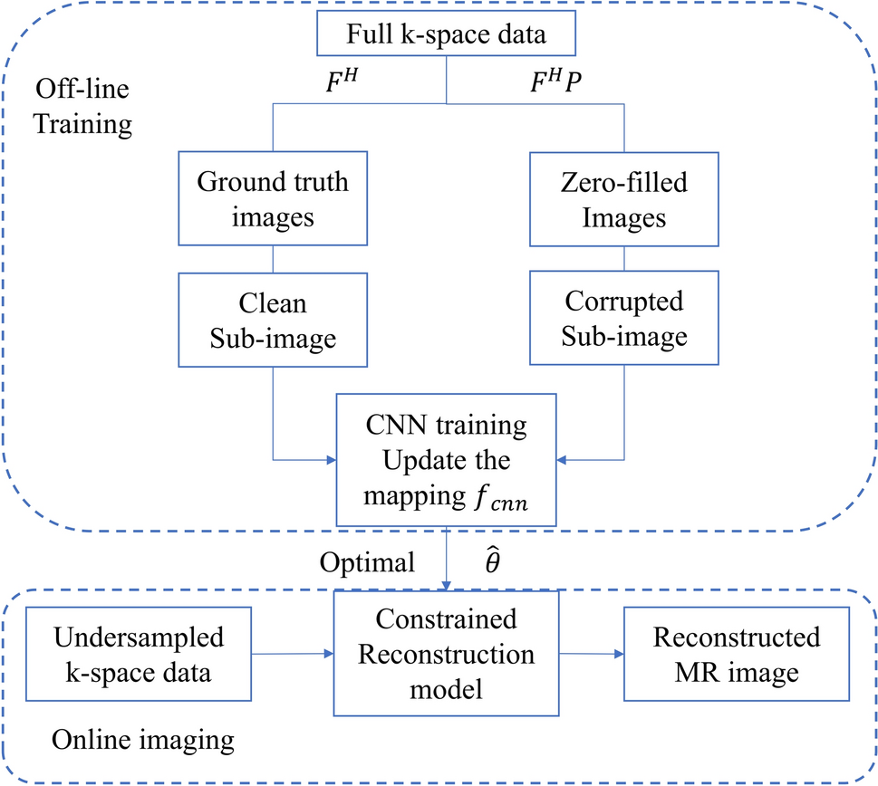
Subspace constrained reconstruction

If \(\Omega _\) is the k-space domain indexed by multi-dimensional index \(\varvec\), ||.|| represents number of elements in the domain, the matrix \(\varvec_c \in \mathbb ^|| \times J}\) contains predictions of the measurements performed with one of the coils out of C indexed by \(c= [1, C]\) and is defined as

$$\begin \varvec_ = \varvec \odot \varvec} \varvec_} \varvec, \end$$

(4)

where \(\varvec \in \^\) is the binary matrix representing an undersampling mask, \(\odot\) represents element-wise multiplication, \(\mathcal \) is the Fourier operator, \(\mathcal _ \in \mathbb ^\) is a diagonal matrix with with the sensitivity for channel c, and \(\varvec \in \mathbb ^\) denotes the echo images. The principle behind the SCR is the low-rank nature of the echo images \(\varvec\), which allows them to be approximated as

$$\begin \varvec = \varvec \varvec, \end$$

(5)

where \(\varvec\in \mathbb ^\) is called a subspace basis function and \(\varvec \in \mathbb ^\) are the coefficients of the subspace where \(d < J\) represents the number of subspace components used. \(\varvec\) primarily should be designed, such that the difference \(\varvec - \varvec \varvec\) is small for all realistic \(\varvec\). From Eqs. 4 and 5, \(\varvec_\) can be written as

$$\begin \varvec^_ = \varvec \odot \varvec} \varvec_} \varvec \varvec. \end$$

(6)

The reconstruction of \(\varvec\) can be formulated as a maximum-likelihood estimation to recover \(\varvec\) from noisy measured k-space data from each coil \(\varvec_ \in \mathbb ^|| \times J}\). The noise in the measured k-space can be assumed to be normally distributed with independent real and imaginary channel. If the variance of noise is \(\sigma ^2\), the estimation problem can be defined by

$$\begin \hat} = \arg \max _} L(\varvec) = \arg \min _} \frac \sum _^ || \varvec_ - \varvec_^ ||_2^2. \end$$

(7)

After estimation of \(\hat}\), echo images \(\varvec\) can be computed using Eq. 5. Note that by defining \(\varvec\) in terms of \(\varvec \varvec\), the number of unknowns decreased from J per voxel to d per voxel. The magnitude of \(\varvec\) can then be used for estimating \(s_}\) for each voxel using the NNLS algorithm proposed by Mackay et al. [9] and further developed to enable B1 inhomogeneity correction by Prasloski et al. [39].

Dictionaries

Various dictionaries \(\varvec\) have been proposed to derive \(\varvec\) by taking SVD of \(\varvec\). Some are data driven [25, 41] and others use a model of signal evolution across echoes [28]. Moreover, different values of d have been used for each application [28]. We describe the selection of \(\varvec\) and d in the following subsections.

Model-based dictionary (\(\varvec^}\))

An analytical model predicts the possible signal evolution for the expected distribution of tissue parameters. For MWF mapping, the multi-component relaxation model defined in Eq. 2 can be used to create dictionary \(\varvec^}\). The change in signal \(\varvec_}\) due to each component can be computed by taking the partial derivative with respect to each of them as shown by Eq. 8 [42]. For a given range of \(T_2\) and the acquisition setting \(\varvec}\), a dictionary \(\varvec^}\) can be produced

$$\begin \begin }^}_ = \frac^}_} }} }. \end \end$$

(8)

Dictionary from fully sampled patch (\(\varvec^}\)) Petzscher et al. [25] proposed to acquire ‘training data’ in the same scan to build a dictionary for \(T_1\) and \(T_2\) mapping. A fully sampled patch in the center of k-space acquired for each echo to produce low-resolution echo images. These low-resolution images can be used as the dictionary \(\varvec^}\).

Selection of dictionaries and number of subspace components

As metric to select the best result among the different dictionaries and number of subspace components (d), we used root-mean-square difference (RMSD) with respect to the reference images or maps (which one will be clear from context)

$$\begin \textrm = \sqrt_|}} \in \Omega ^_} \left( _} - _}\right) ^2}}, \end$$

(9)

where \(\varvec \in \mathbb ^}\) and \(\varvec \in \mathbb ^}\) represent maps or images taken from the region of interest \(\Omega ^_ \subset \Omega _\).

Fig. 1

The two proposed strategies for undersampling 3D-GRASE scans with two GE around each SE are used in this work. The cylinders show frequency-encoding lines. The green color represents the first GE, blue represents SE, and yellow represents the second gradient echo

Accelerating 3D-GRASE sequence

This section starts with a brief description of the state-of-the-art accelerated 3D-GRASE scan proposed by Piredda et al. [18]. Unlike their approach, we intend to exploit redundancy across echoes using SCR additionally to the parallel imaging-based redundancy. Therefore, in the subsequent subsections, we propose two ways to configure the 3D-GRASE for undersampled acquisitions, such that it is more suited for joint reconstruction of echo images.

Accelerated 3D-GRASE state-of-the-art (\(\textrm_0\))

Piredda et al. [18] used parallel imaging to reconstruct images from an undersampled 3D-GRASE scan. As illustrated in Fig. 1, they used the conventional configuration of 3D-GRASE, where two GEs were used along with the SE to sample the same k-space. However, they undersampled the scan further using the CAIPIRINHA undersampling pattern [43]. They used the same undersampling pattern across the echoes. We refer to such approaches where SE and GEs are recorded in the same k-space and the same undersampling pattern is used in each echo as \(\textrm_0\). The B0-inhomogeneity correction was performed using the zero-phase encodes [17, 18].

Accelerated 3D-GRASE 1 (\(\textrm_1\))

As shown in Fig. 1, for this acceleration strategy, we propose to use a distribution of GE and SE similar to \(\textrm_0\); however, we sample different points in k-space for each echo. We refer to such approach as \(\textrm_1\). Using a different undersampling pattern for each echo would promote information sharing across the echoes, which is suitable for joint reconstruction.

We used a low-discrepancy pseudo-random sampling pattern generated using a Halton sequence that was shown to be time-efficient for 3D-GRASE scans [44] referred here after as \(\textrm^\textrm_\). As additional comparison, we also use CAIPIRINHA undersampling pattern [43], which is shifted along one of the spatial dimensions by one position along the echoes referred to as \(\textrm^\textrm_\). Similar to \(\textrm_0\), the B0-inhomogeneity correction was performed using the zero-phase encodes.

Accelerated 3D-GRASE 2 (\(\textrm_2\))

As shown in Fig. 1, in the \(\textrm_2\) configuration, we use GE and SE to fill different k-spaces. Without undersampling, this would require three times the amount of data to fill all k-spaces compared to the MSE scan in the same scan time. However, we propose to undersample each k-space, so that the overall scan time is the same or shorter than the conventional 3D-GRASE scans. We use the Halton sequence and shifted CAIPIRINHA for generating an undersampling pattern similar to \(\textrm_1\) and refer to it as \(\textrm^\textrm_2\) and \(\textrm^\textrm_2\), respectively.

The \(\textrm_2\) configuration requires the model to consider the difference between GE and SE for dictionary generation. The signal from a single voxel in such cases can be modeled as [14, 45]

$$\begin ^_, j} = ^_, j} e^|^}_}} + i}_} } }, \end$$

(10)

where \(\Delta _\) is the time offset of echo \(j = [1,J]\) from the spin echo, \(^}_}\) is the component of \(}^_}\) accounting for the de-phasing of magnetisation and \(\Delta _}\) is the local offset in the main magnetic field. Note that in this case, the number of echoes \(J^_2} = nSE \times (nGE+1)\) where nGE is number of gradient echoes present with each spin echo.

To construct the model-based dictionary for \(\textrm_\), a similar approach as in Eq. 8 is taken where additionally, realistic values of \(\Delta _}\) and \(^}_}\) are taken

$$\begin \begin ^, \textrm_2}_ = \frac_}}} } =&^}_e^|^_}} + i_}}\Delta _ }}. \end \end$$

(11)

Note that we now rename the model-based dictionary defined by Eq. 8 as \(}^}\) to distinguish the dictionaries between \(\textrm_1\) and \(\textrm_2\). We use extended phase graph simulations to compute \(}^}\) [39]. To add \(B_1\) variations to the dictionary, we introduce flip angles (FA) variations in the range from \(120^\circ\) to \(180^\circ\).

B0-inhomogeneity correction A realistic range of B0 values in the dictionary generation step can lead to non-compact subspaces (large d). We hypothesize that by compensating the majority of the B0 effect, the dictionary can be more compact again. Specifically, we propose a B0-inhomogeneity compensation step for \(\textrm_2\) similar to the approach proposed by Liu et al. [46]. A patch of fully sampled region (\(12 \times 12\)) is acquired from the center of the k-space for each echo similar to those required for constructing \(}^}\). We use the patch of fully sampled region to generate low-resolution images \(\varvec}}\). The phase changes observed for voxel \(\varvec\) across the echoes \(j-1\) and j, i.e. \(\angle }_, j-1}} - \angle }_, j}}\), were used to compensate for the effect of B0-inhomogeneities by decreasing the phase changes across the GE and SE images during reconstruction. An experiment to verify how much of overall \(_}\) can be computed using the patch of k-space and the resulting compression in the corresponding subspace is provided in the appendix A.

Experiments

We performed experiments to investigate the accuracy of images, MWF, and \(\textrm_\) maps from SCR images using retrospectively and prospectively undersampled 3D-GRASE acquisitions. Both phantom and in-vivo experiments are performed as described in the following subsections.

Phantom data

We acquired a fully sampled scan of the ISMRM model 130 phantom [47]. The acquisition was performed with a 3.0 T clinical scanner (Discovery MR750, GE Healthcare, Waukesha, WI) with a 32-channel head coil. The acquisition settings are similar to Piredda et al. [18] and given in Table 1. The repetition time (TR) was set to 1800 ms instead of 1000 ms [18] due to a SAR limit of the scanner. The total scan time was 5 h and 23 min. To accommodate the phase correction technique of \(\textrm_0\) and \(\textrm_1\), a single echo train with zero-phase encode amplitude was acquired prior to the echo trains with readout.

Table 1 Acquisition settings used in the phantom and volunteer scans. Note that the integer inside the round brackets for acceleration factor denotes part of the overall acceleration achieved by sampling k-space with SE and GE. Dimensions: FE = frequency encode, \(PE_1\) = phase encoding 1, and \(PE_2\) = phase encoding 2

Reference SE Reference images were constructed from each of the fully sampled SE echoes. For each echo, a complex valued image was reconstructed by FFT and coil combination with coil sensitivity maps obtained via the ESPIRiT technique [48] by BART [49] on the first SE.

Experiment 1

In this experiment, we compare retrospectively undersampled \(\textrm^\textrm_\) and \(\textrm_\), with an overall acceleration factor of 3 (\(R=3\)). The purpose is to observe if any artifacts occur in \(\textrm_\) due to the mixing of SE and GE in k-space and if \(\textrm_\) produces results similar to the reference SE. \(\textrm_\) configuration with \(R = 3\) represents a conventional 3D-GRASE scan where a fully sampled k-space is formed using two GEs around each SE to fill a k-space. We used the same reconstruction technique as the reference SE for \(\textrm_\). For \(\textrm_\), we reconstructed the echo images using SCR with \(\varvec^, \textrm_}\), which was created with the scan settings listed in Table 1. This includes 40 logarithmically spaced \(T_\) values between 15 ms and 2000 ms, 30 logarithmically spaced \(T^_\) values between 10 ms and 1000 ms, and 200 entries of \(_}\) between (-150, 150) Hz. We visually compared the resulting images, specifically looking for artifacts related to SE and GE mixing in \(\textrm_\) and any artifacts due to undersampling in \(\textrm_\) configuration.

Experiment 2

This experiment evaluates the quality of the echo images for three configurations \(\textrm_0\), \(\textrm^\textrm_1\) and, \(\textrm^\textrm_\) and four accelerations factors \(R \in \\). The configurations were retrospectively undersampled from the fully sampled reference scan. A fully sampled region of \(12 \times 12\) was left in the center of the k-space in each echo in the undersampling patterns. The reconstructed images are shown, and the RMSD computed using the magnitude images is used to evaluate the quality with respect to the reference SE images.

The reconstruction for \(\textrm_0\) configuration was performed for each echo separately using ESPIRiT reconstruction technique with the BART toolbox [48, 49]. Note that this differs from the original work, where online reconstruction was performed in the scanner using GRAPPA [18].

The \(\textrm^\textrm_\) and \(\textrm^\textrm_\) configurations were reconstructed using SCR based on \(\varvec^, \textrm_}\) and \(\varvec^, \textrm_}\). The \(\varvec^}\) was the same as described previously for the case of \(R = 3\) except for the range of \(_}\), which was between \((-20, 20)\) Hz.

In-vivo dataFully sampled data

We conducted two fully sampled scans acquiring the complete set of GE and SE on two healthy volunteers (1 and 2) using the same scanner as phantom experiment with settings shown in Table 1 for retrospective undersampling experiments. These acquisitions focused on seven central brain slices to limit scan time. Additionally, a \(T_1\) weighted image was acquired using a 3D FSPGR sequence (Table 1).

Reference data Conventional inverse Fourier transform-based reconstruction was employed (Sect. 2.4.1), and SEs from this experiment served as a reference. We applied the MWF mapping procedure using the same NNLS fitting settings as Piredda et al. [18] with FA ranging from \(120^\circ\) to \(180^\circ\) in \(1^\circ\) increments, obtaining MWF and \(\textrm_\) maps.

Experiment 3

This experiment evaluates the quality of the MWF and \(\textrm_\) maps for three configurations \(\textrm_0\), \(\textrm^\textrm_1\), and \(\textrm^\textrm_2\) and six accelerations factors \(R \in \\) by retrospectively undersampling the fully sampled data. We selected the central slice (no. 4) from the reference scan. We treated Anterior–Posterior and Left–Right as \(PE_1\) and \(PE_2\) for retrospective undersampling experiments, generating \(\textrm_0\), \(\textrm^\textrm_\), \(\textrm^\textrm_\), \(\textrm^\textrm_2\), and \(\textrm^\textrm_2\) with overall accelerations of \(R \in \\) from both the volunteer scans. For computing the coil maps and the \(\varvec^}\) in case of \(\textrm_1\), a \(12 \times 12\) patch in the center of k-space in each echo was left fully sampled.

The retrospectively undersampled data for volunteer 1 were reconstructed using all possible dictionary and subspace component combinations. We reconstructed the SE and GE images from one volunteer scan using the same process as the reference SE data from the phantom experiment described in Sect. 2.4.1.

The \(T_1\) weighted images were processed by Freesurfer [50] to create a segmentation mask. The \(T_1\)-weighted images were registered to the echo image 14 of the slices of reference scan using FSL toolbox [51]. The white matter mask from the segmentation was transformed into the space of the reference scan. The masks were used as ROI to compute RMSD between accelerated maps and reference maps. The dictionary and the number of subspaces with the lowest RMSD were used to reconstruct the volunteer 2 data for each configuration, undersampling pattern, and acceleration factor.

Experiment 4

We tested the possibility of prospective undersampling. We performed a prospectively undersampled scan on a single healthy volunteer (3) using three different configurations: \(\textrm_0\), \(\textrm^\textrm_1\), and \(\textrm^\textrm_2\). The overall acceleration factor was \(R = 9\) including a fully sampled 12 x12 center patch. Excluding that patch the acceleration factor was \(R = 12\). Further acquisition settings are given in Table 1. Additionally, we obtained a fully sampled scan with seven slices from the central region of the brain for comparison. We aligned the central seven slices of the accelerated and reference scans based on their world coordinates during the scan. The dictionary and number of subspace components were selected based on the results of Experiment 3. A \(T_1\) weighted image was acquired and used for tissue segmentation as in Experiment 3 and registration to image \(t = 14\) (E = 140 ms) of the \(\textrm_0\) scan. The white matter mask from the segmentation was warped with the registration result to form a region of interest in which the RMSD between reference and accelerated scans is evaluated.