In this study, the effects of excluding fatty tissue in QSM reconstruction of the knee were evaluated from in vivo data. Three masking alternatives were compared: (1) excluding no tissue, (2) excluding bone marrow, and (3) excluding all fatty tissues. For all masking options, the chemical shifts of multiple fat frequency components were addressed using CSEI. QSM reconstruction was made using morphology enabled dipole inversion (MEDI) [22,23,24,25], comparing three background field removal techniques: variable-kernel sophisticated harmonic artifact reduction for phase data (V-SHARP) [26], projection onto dipole fields (PDF) [27], and Laplacian boundary value (LBV) [28]. In addition, results in the medial and lateral tibiofemoral compartments were compared.

All data analysis and post processing were performed using MATLAB [The MathWorks Inc. (2023). MATLAB version: 9.8 (R2020a) Natick, MA USA]. The data acquisition and analysis are summarized in Fig. 2.

Fig. 2

A flowchart describing the steps performed in the acquisition and post processing of data for QSM reconstruction. The processing steps where masks were applied are indicated by *

Human subjects

Image data from 23 participants without known OA were collected with permission from the ethics review authority and after written informed consent. For each participant, the knee to be imaged was selected randomly. Before image acquisition, a Knee Osteoarthritis Outcome Score (KOOS) questionnaire was filled out by each participant. Based on the KOOS scores, asymptomatic subjects were identified as described in Ref [29]. Briefly, 42 questions separated into five categories (quality-of-life, pain, symptoms, activities of daily living and sport and recreation function) were answered using a five-grade scale. The answers were converted to five scores between 0 and 100, where a lower score indicated more severe OA symptoms. Scores below a defined cutoff for quality of life and any two of the other categories were taken as an indication of a symptomatic knee, see cut-off values for each category in ref [29]. In this analysis, which was part of a larger study, only data from asymptomatic participants were included. Further, one subject was excluded due to the presence of red bone marrow resulting in a low fat fraction of the femoral bone marrow and four subjects were excluded due to fat/water swaps in the CSEI reconstruction. This yielded data from a total of 18 participants, 6 men and 12 women, aged between 34 and 61 years (mean 47.3 years).

Image acquisition

Image acquisition was performed on an actively shielded 7 T Philips MR system (Achieva, Philips Healthcare, Best, NL), using a QED Knee Coil 1TX/28RX (Quality Electrodynamics LCC, Mayfield Village, OH USA), step 1 in Fig. 2. Two sagittal and interleaved multi-echo gradient echo sequences, each with bipolar read-out gradients and eight echo times, such that TE1, sequence 1/ΔTE = 1.2/1.2 ms and TE/ΔTE = 1.8/1.2 ms, were collected and combined, yielding ΔTEeffective = 0.6 ms. The following parameters were used: TR = 30 ms, matrix size = 256 × 256 × 37, voxel size = 0.58 × 0.58 × 3 mm3, flip angle = 8°, SENSE acceleration factor = 1.2, and bandwidth = 1378 Hz/pixel. The phase and magnitude of the signal was obtained along with a B0 map from the mDixon Quant application (Philips Healthcare, Best, NL).

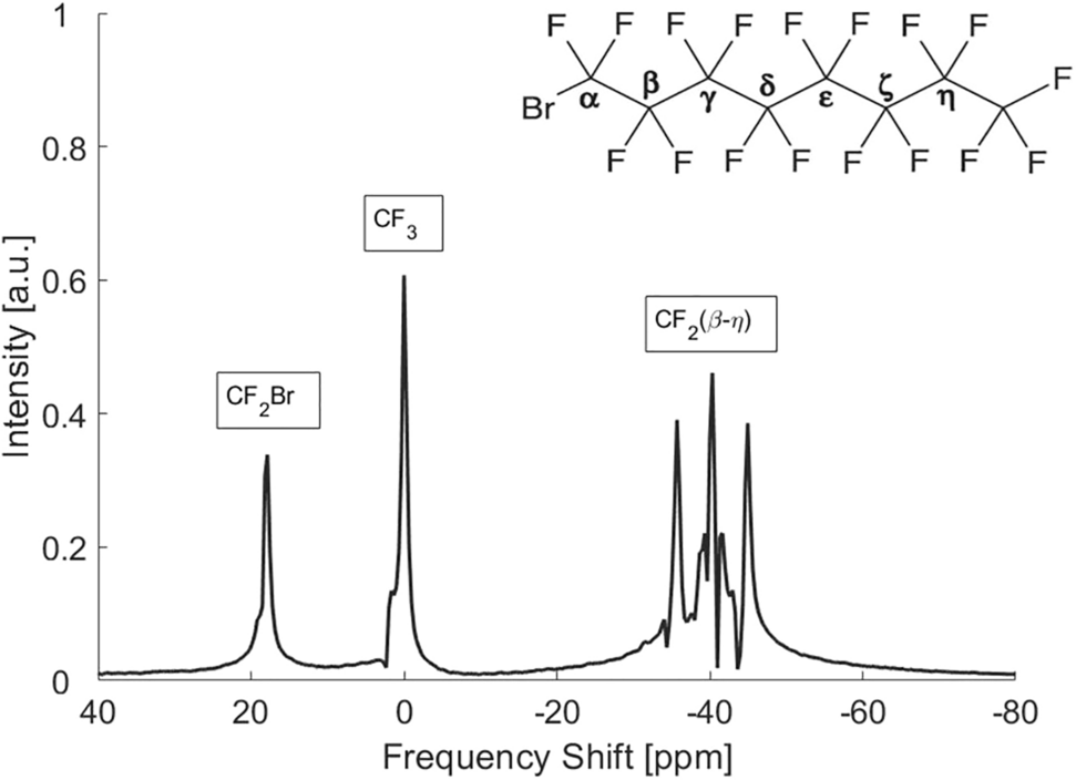
Data processing and reconstruction of susceptibility mapsChemical shift encoded imaging

Based on the collected data, a proton density fat fraction map (PDFF), and a chemical-shift corrected total field perturbation map (ΔBtot), was calculated for each participant using CSEI (step 2 in Fig. 2). The iterative linear least-squares reconstruction included an a priori fat model with M = 8 peaks with relative amplitudes \(_\) and frequency differences compared to water \(\Delta _\), as well as estimation of R2* and phase errors due to the interleaved \(_}\) and bipolar \(_}\) acquisition [30, 31], using the following signal equation:

$$\beginS\left(TE,n,p\right)=\left(W+F\sum_^_^_TE}\right)^^^i\pi _}^_}},\end$$

(1)

where W and F denote water and fat, n the number of the echo in each echo train, and p = − 1 for the first interleave and p = 1 for the second interleave. Here, the \(\Delta _}\) and R2* are obtained from the real and imaginary part of the complex field map \(\psi\), according to [32]

$$\begin\psi =\Delta _}+\frac^}.\end$$

(2)

The complex field map is constructed, such that

$$\begin^=^_+\frac^}\right)TE}=^_}^^TE}.\end$$

(3)

The mDixon B0 map, in some cases slightly shifted in frequency to avoid fat–water swaps, was used as an initial guess. Also, an R2*-map was calculated using the ARLO function [33] from the MEDI toolbox [22,23,24,25].

Segmentation and mask definition

For each participant, three masks were defined (step 3 in Fig. 2):

(1)

excluding no tissue: obtained by thresholding based on the magnitude image collected with TE = 1.2 ms.

(2)

excluding bone marrow: obtained by defining bone marrow regions and excluding them from the first mask. This was done by first defining all fatty tissues using a threshold level of PDFF > 70%. From this, bone marrow in femur, tibia, fibula, and patella was separated from other fatty tissues using region growing in the R2*-map.

(3)

excluding all fatty tissues: obtained by thresholding voxels with a fat fraction larger than 35% in the PDFF map, and excluded from the first map.

Threshold values in the magnitude and PDFF images were determined based on visual inspection of images. In some cases, manual corrections of masks were needed to ensure satisfactory definition of the tissues. Extra attention was given to make sure that: (1) air was not included in the mask, (2) a good correspondence was obtained between the marrow regions of the mask and the marrow regions of the PDFF maps, and (3) the articular cartilage between femur and tibia was not lost.

QSM reconstruction

The chemical-shift corrected total field perturbation map ΔBtot from CSEI was used to calculate the magnetic susceptibility using the MEDI toolbox. First, background field removal was performed with each of the three techniques, V-SHARP, PDF, and LBV, yielding the local field perturbation (ΔBlocal), see step 4 in Fig. 2, where V-SHARP was used via SEPIA [34]. For all, standard settings were used with the following exceptions: (1) For PDF, the maximum number of iterations was set to 100, and (2) for V-SHARP, a minimum radius of 1 mm and a maximum radius of 10 mm were used.

Second, dipole inversion was performed using MEDI with a regularization parameter λ = 200; see step 5 in Fig. 2.

Erosion of the mask was performed throughout the reconstruction steps, to minimize artifacts stemming from the edge regions [35]. Around the air–tissue interface, an erosion of three pixels was performed before background field removal, and an erosion of two pixels before the dipole inversion step. At the fatty–lean tissue interface, however, smaller erosion was necessary to avoid loss of the articular cartilage volume. Here, erosion of only one pixel was performed before each of the background field removal and dipole inversion steps.

Data analysis

In each susceptibility map, rectangular regions of interests (ROIs) with an anterior–posterior width of five pixels were defined in one medial and one lateral slice, respectively, covering the articular cartilage between the femoral and tibial bone surfaces. In each ROI, the susceptibility values were shifted by addition/subtraction, so that the value at the cartilage surface was set to zero to make it possible to visually compare the relative susceptibility values obtained from QSM. Each ROI was manually divided into a femoral and tibial part based on magnitude data.

Susceptibility profiles were visualized by plotting susceptibility values within ROIs against the relative distance from the bone surfaces, see Fig. 1b. As no ground truth was known, and could thus not be used for comparison, the results were evaluated based on two assumptions: (1) that susceptibility should increase with distance from the bone surfaces [6, 7] and (2) that the profile over the cartilage should be constant within subject and compartment, and thus not affected by the choice of masking method. The quality of the susceptibility profile for each participant and for each of the femoral and tibial compartments was thus evaluated using two measures; see Fig. 1b.

First, the slope of a linear regression between susceptibility and relative distance from the bone surface was used as a measure of contrast between cartilage layers [ppm/%]. A positive slope indicates the expected increase in susceptibility values going from the bone to the cartilage surface. Assuming a linear relationship between susceptibility and relative distance from the bone surface is a simplified model of the complex cartilage structure but is motivated by the low imaging resolution and thus few data points available in each compartment.

Second, Pearson’s correlation coefficient was estimated and used in two ways. First, as an indication of whether a linear model is a reasonable description of the association between susceptibility and distance from the bone surface in vivo, and second, to evaluate to what extent unexpected susceptibility profiles were present, which may possibly be related to artifacts in the QSM images.

The methods were compared using a Bland–Altman analysis, using the masking alternative of excluding no tissue with V-SHARP background field removal as a reference. For each comparison, the average difference and upper and lower limit of agreement (LoA) were estimated with 95% confidence interval (CI).