Ethical approval was granted from OxTREC ethics committee at Oxford, REF: R90824/RE001. Main analyses were pre-registered prior to collection of the data [25]; full details in Supplement 4.

Sampling

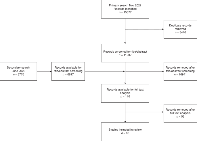
To elicit preferences of GPs, 251 GPs were recruited by M3 Group, who recruit medical professionals for surveys. They used email lists that GPs had signed up to. We included GPs that were currently practising in England. Quotas (age, gender, and region), based on the NHS General Practice Workforce data, were used to increase representativeness. 6757 GPs were invited to participate in the survey. 812 started the survey, 66 failed eligibility, 104 exceeded the maximum time limit, and 391 were in excess of the quotas (and did not complete the survey); see Supplement 3 for further details. GPs were rewarded with credits on M3’s platform equivalent to a GP’s hourly rate pro-rated to the expected survey time of 15 min.

With regards to public preferences, 1005 members of the general public were recruited by SurveyEngine, a survey company that provides panels in the UK. They used email lists that individuals signed up to. We included adults (18 years or older) living in England. Quotas (age, gender, and region) based on the UK census, were used to promote representativeness. 1465 individuals were invited to participate in the survey. 1413 started the survey, 70 failed eligibility, 158 exceeded the maximum time limit, 7 failed the minimum time limit (less that 1/3 of the median time taken in the pilot study), 4 failed open-ended sense response checks (i.e. gave erratic responses), and 169 were in excess of the quotas (and did not complete the survey); see Supplement 3 for further details. Individuals were rewarded with credits on SurveyEngine’s platform equivalent to the UK minimum wage pro-rated to the expected survey time of 15 min.

Discrete choice experiment (DCE)

A DCE is a technique used widely in health to understand preferences by asking participants to make specific choices [26, 27]. Here, participants were presented with a choice between two MCTs. Each test was defined by a set of attributes, such as whether the test can identify the cancer site, and the variation in each attribute (in this example, “yes” or “no”) is referred to as a level. By making a series of choices between a hypothetical MCT with one set of attributes and levels and another MCT with alternative attributes and levels, participants implicitly reveal the degree to which each attribute is important to them and the value they place on each level of the attribute.

The two DCEs, one for each stakeholder group, were designed according to experimental best practices, ranging from design efficiency to participant-centred aspects such as checking experimental tasks were clear to participants [28, 29]. Individuals made 12 choices between two hypothetical MCTs. The alternatives were described by attributes and levels (below) representing different hypothetical MCTs.

Attributes and levels

Seven attributes described the characteristics of MCTs in the choice tasks, summarised in Table 1. The full descriptions, as presented to respondents, are provided in supplement 1. Attributes and levels were selected based on several sources of evidence: a scoping review of choice experiments including diagnostic technologies (see Supplement 12 for details); collaborative working with clinical experts on the study team; and a group interview with members of the public (n = 4).

Table 1 Descriptive system: attributes and levels used in the discrete choice experiment.PPIE input into the design

A focus group with 4 members of the public helped to maximise understanding of the experiment by discussing drafts and refining the descriptions of the attributes. For example, the attribute of number of cancer sites tested for was reworded to “number of cancers tested for” for members of the general public as this was clearer to focus group participants (though not for GPs since this terminology is routine to them). This group agreed that communicating test accuracy in three ways (rhetorically, numerically, and graphically), rather than just numerically, would maximise respondents’ understanding. In addition, PPIE contributors found the concepts of sensitivity and specificity difficult to understand despite various options being presented to them. They found explanations of predictive values easier to comprehend when expressed as the accuracy of a positive or negative test. We therefore opted to include attributes about positive and negative test accuracy in both patient and GP DCEs to allow comparison between the two groups. All information was framed to increase understanding, drawing on this qualitative work and public input.

Pilot phase with members of the public

We conducted a pilot study in members of the public (n = 62), in which we asked respondents to report misunderstandings and/or difficulties, and adjusted questions as required. None of the respondents reported difficulties in understanding and none reported any discomfort in taking the survey. The attribute levels were altered from the analysis plan following the analyses of the pilot data. These alterations were intended to improve understanding and efficiency: (i) The form of the test attribute levels “saliva” and “oral swab” were removed. In the pilot data, there was no evidence to suggest that the levels “saliva” or “oral swab” were impactful on test preferences therefore these levels were removed from the final design. (ii) The negative test accuracy attribute levels for GPs were changed from 6 to 4 levels. The attribute for negative test accuracy for GPs had one level removed to simplify and balance the design so that each level for each attribute appears the same number of times. (iii) Randomisation of members of the public to positive or negative predictive value attributes. From the PPIE focus groups and pilot data, it became clear that expressing test accuracy both positively and negatively simultaneously was confusing. Keeping both of these attributes in a single DCE would likely result in poor quality data because comprehension would be low. We switched to a split design (Hess et al., 2017), where half of the public sample would be randomly allocated to a design with PPV, and the other half to NPV; all other attributes and levels were the same in both arms. Hence, each patient’s choices were described by 6 attributes, and preferences for the full set of 7 attributes were subsequently modelled by combining the arms and applying appropriate statistical corrections (see later section).

Experimental design

A Bayesian D-efficient design was generated that contained 24 choice tasks. Priors were obtained from the pilot study. For GPs, the tasks included 7 attributes. For members of the public, two versions of choice tasks (where respondents were randomised to either a positive or a negative predictive value) were generated from the same design. This design used two utility functions, one each for each choice task version, and averaged over those versions. In both samples, individuals were randomized to two blocks of 12 choice tasks, balancing concerns of learning and respondent fatigue [29]; that is, to keep the number of tasks manageable for respondents. Examples of choice tasks, and the schematic for randomization through the survey, are presented in Supplement 2.

Survey

The online survey was distributed through email lists, accompanied by an introductory letter and instruction sheet. The questionnaire, tailored to each sample, collected sociodemographic information (both samples), experience and knowledge of cancer (general public sample), practice characteristics (GP sample), and validation questions at the end of the survey to assess the quality of their responses. Public cancer knowledge and experiences were assessed using a set of questions in the survey, including how many symptoms of cancer individuals could identify from a list, whether the individual had ever had cancer, whether the individual had ever been tested for cancer, and whether the individual had ever been screened for cancer. They were asked further questions on their health behaviours (smoking, exercise, etc.).

Data quality

Respondents were given narrative and visual information describing the alternatives, attributes, and levels. A practice choice scenario was presented prior to the main experiment. “Forced responses” prevented respondents from skipping past questions in the survey; and a minimum time threshold of 2.5 min, based on pilot data, removed respondents who rushed through. Duplicate survey responses were rejected. Open-ended text responses were examined and suspicious responses (such as “October” given as an answer to a cancer estimate question) were identified and removed [30]. A post-experiment question asked respondents which attribute was most important. This allowed us to assess internal validity by checking for consistency with the model estimates.

Statistical analyses

Our sample size was sufficient to ensure statistical power based on the pilot parameter estimates [31].

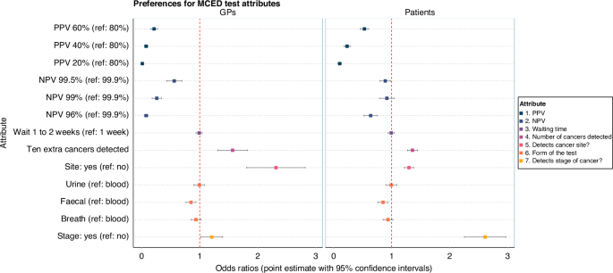
Primary analyses used mixed multinomial logit models to analyse the impact of attribute levels on experimental choices. The dependent variable in the regression models was the selection of the hypothetical tests, “MCT 1”, or “MCT 2”. Attributes were independent variables. Attributes were dummy-coded [32]. Odds ratios were computed by exponentiating the estimated coefficients.

Data from the GP and public samples were pooled and modelled jointly. A first scale parameter adjusted for the public randomisation to either the positive or negative predictive value. A second scale parameter adjusted for differences between the GP and public experimental layout (e.g. wording differences of the same attributes between the two designs). Sample weighting was applied in the regressions to account for the unequal size of the two samples (the sample of public was four times larger than the sample of GPs). A set of interaction terms were specified using a “sample” dummy (i.e. GP or public sample) and the attributes.

Marginal rates of substitution (MRSs) were computed for NPV and PPV for both GPs and the general public, these being the ratios of estimated parameters (delta method applied to compute confidence intervals). MRSs reflect the relative value of PPV and NPV. More specifically, MRSs give the amount of PPV that would be needed to compensate for a lower NPV between two MCTs, such that they are considered as good as one another (all else being equal).

Secondary analyses assessed preference variation in the overall sample across a set of demographics using interaction terms: age, gender, ethnicity, education, and urbanicity. For deterministic heterogeneity, a refining procedure specified models with all interactions and iteratively removed non-significant parameters from each model. A factor analysis was performed to investigate patterns of correlation between public cancer knowledge and experiences, and the results of this analysis guided the construction of a latent variable of cancer knowledge and experience. In measurement equations of the latent variable, each question was treated as an outcome and the latent variable was the explanatory variable. Using a structural equation, the latent variable was regressed on a set of individual covariates (i.e. age, gender, ethnicity, education, and rurality) to understand how cancer experience varies across demographics. Finally, the latent variable of cancer knowledge and experience entered the choice model in a similar way to patient demographics, to relate attribute preference variation with patient knowledge and experience of cancer. This model extends the mixed multinomial logit using a system of equations that is simultaneously estimated, and known as Integrated Choice and Latent Variable (ICLV) model [33]. See supplement 4 for details and a diagram of the system of equations.

Statistical significance was examined with t-ratios (i.e. two-tailed t-tests). Models were estimated using the Apollo package in R [34]. Code scripts are available on request.

Simulations for ranking MCTs

It is possible to simulate choices for any combination of attributes by setting the attribute values in the data and applying these to the model. In this way, we predicted probabilities of choosing all possible MCTs based on all the combinations of attribute levels in the design (n = 2048). By taking any one MCT and using it as a comparator (i.e., benchmark), we can rank the entire set of MCTs relative to that comparator. In this case, we used the characteristics of GRAIL’s Galleri MCT as reported in the SYMPLIFY study for comparison as, at the time of writing, it was only MCT with published data from a symptomatic population (hereafter named the ‘SYMPLIFY MCT’) [21]. In addition, we compared preferences for simulated MCTs with the features of cancer diagnostics currently used in primary care practice: the faecal immunochemical test (FIT); prostate-specific antigen (PSA) test; and the CA125 blood test. Technical details, and details of the MCTs, are provided in Supplements 4 and 5.