In the following, we shall assume that the Lie algebra \(\mathfrak \) also comes with an (invariant) metric \(\langle -,-\rangle \).

3.1 CR Ambitwistor Action

CR Holomorphic Volume Form. To write down a Chern–Simons-type action, we need to construct an appropriate volume form. To this end, we consider the twisted CR holomorphic differential form

$$\begin \omega _}\ :=\ v^\textrm\wedge v^\textrm\wedge v^}}\wedge v^\textrm\wedge v^\textrm\wedge \textrm\eta _1\wedge \textrm\eta _2\wedge \textrm\eta _3\wedge \textrm\theta ^1\wedge \textrm\theta ^2\wedge \textrm\theta ^3. \end$$

(3.1)

Note that we may replace \(\textrm\eta _i\) by \(v_i\) and \(\textrm\theta ^i\) by \(v^i\) because of the appearance of \(v^\textrm\) and \(v^\textrm\) and as follows from (2.23).Footnote 27 For the same reason, the terms proportional to \(}^i}_i\) in \(v^\textrm\) and \(v^}}\) drop out. Hence, \(\omega _}\) depends on the fermionic coordinates only via the CR holomorphic combinations \(\eta _i\) and \(\theta ^i\). This allows use now to transition to integral forms by requiring the Berezin integrationsFootnote 28

$$\begin \int \textrm\eta _i\eta _j\ :=\ \delta _ ~~~}\int \textrm\theta ^i\theta ^j\ :=\ \delta ^ \end$$

(3.2)

for the CR holomorphic coordinates. Consequently, we arrive at the integral form

(3.3)

which we call the twisted CR holomorphic volume form. It is now not too difficult to see that because of (3.2), \(\Omega _}\) is of homogeneity zero and thus, globally well defined on F. It is also \(\bar_}\)-closed which is a direct consequence of the commutation relations amongst the vector fields (2.26b) and (2.28a).

CR Holomorphic Chern–Simons Form and Action. Furthermore, the terms proportional to \(\theta ^i\eta _i\) in \(v^\textrm\) and \(v^}}\) in (3.3) also drop out in the wedge product of (3.3) with the twisted CR holomorphic Chern–Simons form

$$\begin \textrm_}\ :=\ \tfrac\langle A,\bar_\mathrmA\rangle +\tfrac\langle A,[A,A]\rangle ~, \end$$

(3.4a)

where now \(A\in \Omega ^_}(F)\otimes \mathfrak \) is taken to be in the Witten gauge (2.37) the latter of which we can always assume by virtue of Proposition 2.5. Therefore, in the Witten gauge, the twisted CR holomorphic Chern–Simons equation (2.34) follows upon varying the twisted CR holomorphic Chern–Simons actionFootnote 29

$$\begin S\ :=\ \int \Omega _}\wedge \textrm_}. \end$$

(3.4b)

Remark 3.1

Note that the action (3.4b) can be understood to live on the real 8|12-dimensional submanifold \(L\rightarrow \mathbb ^4\times \mathbb P^1\times \mathbb P^1\) inside the augmented CR ambitwistor space F with L the pull-back of the fermionic holomorphic vector bundle \([\mathcal (1,0)\oplus \mathcal (0,1)]\otimes \mathbb ^\rightarrow \mathbb P^1\times \mathbb P^1\) to the body \(\mathbb ^4\times \mathbb P^1\times \mathbb P^1\rightarrow \mathbb P^1\times \mathbb P^1\) of F. We shall call L the CR ambitwistor space.

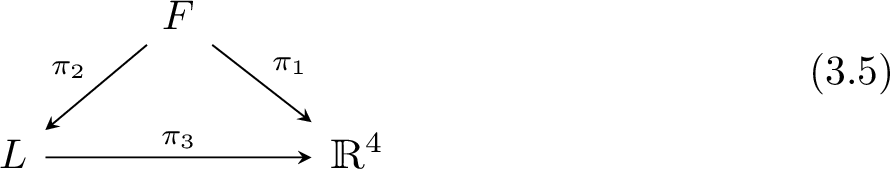
We have the commutative triangle of fibrations

where \(\pi _1\) is the trivial projection \(\mathbb ^4\times \mathbb P^1\times \mathbb P^1\rightarrow \mathbb ^4\), \(\pi _2:(x^},\eta ^}_i,\theta ^,\lambda _},\mu _\alpha )\mapsto (x^},\eta _i,\theta ^i,\lambda _},\mu _\alpha )\) with the tangent spaces of the fibres of \(\pi _2\) spanned by the (commuting) fermionic vector fields \(\hat^i\) and \(\hat_i\), and \(\pi _3\) is the concatenation of the bundle projection \(L\rightarrow \mathbb ^4\times \mathbb P^1\times \mathbb P^1\) and the trivial projection \(\mathbb ^4\times \mathbb P^1\times \mathbb P^1\rightarrow \mathbb ^4\).

Consequently, the twisted CR holomorphic volume form in (3.4b) can be taken to be

$$\begin \Omega _}\ \rightarrow \ \Omega _}\ :=\ e^\textrm\wedge e^\textrm\wedge e^}}\wedge e^\textrm\wedge e^\textrm\otimes \underbrace\eta _1\textrm\eta _2\textrm\eta _3}_^3\eta }\underbrace\theta ^1\textrm\theta ^2\textrm\theta ^3}_^3\theta }~, \end$$

(3.6a)

where now \(e^\textrm\), \(e^\textrm\), \(e^}}\), \(e^\textrm\), and \(e^\textrm\) are as in (2.8). Likewise, the differential \(\bar_}\) in (3.4a) can be taken to be the reduced differential given in (2.35), that is,

$$\begin \bar_}\ \rightarrow \ \bar_\mathrm\ =\ \hat^\textrm\hat_\textrm+\hat^\textrm(\hat_\textrm+\theta ^i\eta _iE_}})+\hat^\textrm(\hat_\textrm+\theta ^i\eta _iE_\textrm)~, \end$$

(3.6b)

where now \(\hat^\textrm\), \(\hat^\textrm\), and \(\hat^\textrm\) are as in (2.8. By construction, \(\Omega _}\) is \(\bar_\mathrm\)-closed.

Batalin–Vilkovisky Action. We may also consider the Batalin–Vilkovisky extension of the CR ambitwistor action (3.4b). This action is obtained by replacing the Lie-algebra valued (0, 1)-form A in the twisted CR holomorphic Chern–Simons form with a general element \(\mathcal \in \Omega ^_}(F)\otimes \mathfrak \). Such an element is of the form

$$\begin \mathcal \ =\ C+A+A^++C^+ \end$$

(3.7a)

with \(C\in \Omega ^_}(F)\otimes \mathfrak \) the ghost, \(A^+\in \Omega ^_}(F)\otimes \mathfrak \) the anti-field of the gauge potential A, and \(C^+\in \Omega ^_}(F)\otimes \mathfrak \) the anti-field of C. In terms of these component fields, the corresponding Batalin–Vilkovisky action reads as

$$\begin \begin S_}\ &:=\ \int \Omega _}\wedge \Big \\langle A,\bar_}A\rangle +\tfrac\langle A,[A,A]\rangle \\&\quad +\langle A^+,\bar_}C+[A,C]\rangle +\tfrac\langle C^+,[C,C]\rangle \Big \}\,. \end \end$$

(3.7b)

3.2 Equivalence to \(\mathcal =3\) Supersymmetric Yang–Mills Theory

Proposition 2.1 shows that the twisted CR holomorphic Chern–Simons equation of motion and the equations of motion of \(\mathcal =3\) supersymmetric Yang–Mills theory are equivalent. In the remainder of this paper, we shall demonstrate that this equivalence extends to the level of the ambitwistor action (3.4b) and its Batalin–Vilkovisky extension (3.7b), culminating in Theorem 3.5. Equivalence here is again precisely the semi-classical equivalence mentioned above, i.e. \(L_\infty \)-quasi-isomorphy. Concretely, the differential graded Lie algebra defined by the CR holomorphic Chern–Simons action (3.7b) and the differential graded Lie algebra defined by the first-order Batalin–Vilkovisky action (3.11) are quasi-isomorphic.

Furthermore, this \(L_\infty \)-quasi-isomorphism can be phrased as a homotopy transfer and thus, physically, corresponds to integrating out infinitely many auxiliary fields in the action (3.7b). For the reader’s convenience, we summarise the key formulas about homotopy transfer in Appendix A.2.

The proof of the corresponding theorems, Theorem 3.5 and Theorem 3.6, is broken down into several steps. Firstly, we give a brief review of the first-order formulation of Yang–Mills theory and its Batalin–Vilkovisky extension. Secondly, we establish that there is a cyclic quasi-isomorphism between the cochain complexes underlying both theories. Finally, we show that this quasi-isomorphism extends to an \(L_\infty \)-quasi-isomorphism between the differential graded Lie algebras governing both theories and that this quasi-isomorphism is a homotopy transfer. To keep the formulas manageable, we shall restrict the explicit parts of our calculations to the R-symmetry singlets of the \(\mathcal =3\) multiplet, that is, to the gluons. The full equivalence follows then from covariance of all our constructions under supersymmetry.

First-Order Yang–Mills Action. As before, let \(\mathfrak \) be a Lie algebra with Lie bracket \([-,-]\) and inner product \(\langle -,-\rangle \). The standard second-order Yang–Mills action is

$$\begin S\ =\ \tfrac\int \textrm^4x\,\Big \\dot},f_\dot}\rangle +\langle f^,f_\rangle \Big \}\,, \end$$

(3.8a)

where

$$\begin \begin f_\dot}\ &:=\ \tfrac\varepsilon ^\big \}A_}-\partial _}A_}+[A_},A_}]\big \}\\&=\ \varepsilon ^\partial _}A_)}+\tfrac\varepsilon ^[A_},A_}]\,, \\ f_\ &:=\ \tfrac\varepsilon ^\dot}\big \}A_}-\partial _}A_}+[A_},A_}]\big \}\\&=\ \varepsilon ^\dot}\partial _}A_}+\tfrac\varepsilon ^\dot}[A_},A_}] \end \end$$

(3.8b)

are the anti-self-dual and self-dual parts of the curvature of the Lie-algebra-valued one-form \(A_}\). Introducing the anti-self-dual, \(B_\dot}=B_\dot}\), and self-dual, \(B_=B_\), parts of an auxiliary Lie-algebra valued auxiliary two-form transforming in the adjoint representation of the gauge group, we can write the first-order action of Yang–Mills theory as

$$\begin S\ =\ \int \textrm^4x\,\Big \\dot},f_\dot}-\tfracB_\dot}\rangle +\langle B^,f_-\tfracB_\rangle \Big \}\,. \end$$

(3.9)

Evidently, upon integrating out \(B_\dot}\) and \(B_\), we recover the second-order Yang–Mills action (3.8a). The equations of motion following from (3.9) read as

$$\begin f_\dot}\ =\ B_\dot}~,~~~ f_\ =\ B_~, ~~~}\varepsilon ^\dot}\nabla _}B_\dot}+\varepsilon ^\nabla _}B_\ =\ 0~, \end$$

(3.10a)

where, as before, \(\nabla _}=\partial _}+[A_},-]\). Because of the Bianchi identity,

$$\begin \varepsilon ^\dot}\nabla _}f_\dot}-\varepsilon ^\nabla _}f_\ =\ 0~, \end$$

(3.10b)

the equations of motion (3.10a) are equivalent to

$$\begin f_\dot}\ =\ B_\dot}~,~~~ f_\ =\ B_~,~~~ \varepsilon ^\dot}\nabla _}B_\dot}\ =\ 0~, ~~~}\varepsilon ^\nabla _}B_\ =\ 0. \end$$

(3.10c)

Furthermore, the Batalin–Vilkovisky extension of the first-order Yang–Mills action (3.9) reads as

$$\begin \begin S_}&= \int \textrm^4x\,\Big \\dot},f_\dot}-\tfracB_\dot}\rangle +\langle B^,f_-\tfracB_\rangle \\&\quad +\langle A^+_},\nabla ^}c\rangle +\langle B^+_\dot},[B^\dot},c]\rangle +\langle B^+_,[B^,c]\rangle +\tfrac\langle c^+,[c,c]\rangle \Big \}\,, \end \end$$

(3.11)

where c is the ghost field, and \(A^+_}\), \(B^+_\dot}=B^+_\dot}\), \(B^+_=B^+_\), and \(c^+\) are the evident anti-fields.

As familiar from the example of Chern–Simons theory, also this action defines a differential graded Lie algebra \(\mathfrak _}\) with the underlying cochain complex

and the binary products \(\mu _2\) defined by

$$\begin \begin&\mu _2(c_1,c_2)\ :=\ [c_1,c_2]~,~~~ \mu _2(c,A_})\ :=\ [c,A_}]~, \\&\mu _2(c,B_\dot})\ :=\ [c,B_\dot}]~,~~~ \mu _2(c,B_)\ :=\ [c,B_]~, \\&\mu _2(c,c^+)\ :=\ [c,c^+]~,~~~ \mu _2(c,A^+_})\ :=\ -[c,A^+_}]~, \\&\mu _2(c,B^+_\dot})\ :=\ -[c,B^+_\dot}]~,~~~ \mu _2(c,B^+_)\ :=\ -[c,B^+_]~, \\&\mu _2(A_},A_})\ :=\ \tfrac\big (\varepsilon ^[A_},A_)}],\varepsilon ^\dot}[A_},A_}]\big )\,, \\&\mu _2(A_},B_\dot})\ :=\ \varepsilon ^\dot}[A_},B_\dot}]~,~~~ \mu _2(A_},B_)\ :=\ \varepsilon ^[A_},B_]~, \\&\mu _2(A_},A^+_})\ :=\ -[A^},A^+_}]~, \\&\mu _2(B_\dot},B^+_\dot})\ :=\ -[B^\dot},B^+_\dot}]~,~~~ \mu _2(B_,B^+_)\ :=\ -[B^,B^+_]. \end \end$$

(3.12b)

One can show that this first-order formulation is semi-classically equivalent to the second-order formulation following the constructions in [26, 74, 75]. The same applies to the \(\mathcal =3\) supersymmetric extension.

Embedding of Theories. Consider the differential graded Lie algebras \(\mathfrak _}\) and \(\mathfrak _}\) defined in (2.36) and (3.12a), respectively, and define a degree-zero morphism of graded vector spaces

$$\begin \begin&\textsf\,:\,\mathfrak _}\ \rightarrow \ \mathfrak _}~, \\&c\ \mapsto \ C~,~~~ \left( A_}\\ B_\dot},B_\end}\right) \ \mapsto \ A~,~~~ \left( A^+_}\\ B^+_\dot},B^+_\end}\right) \ \mapsto \ A^+~,~~ c^+\ \mapsto \ C^+ \end\nonumber \\ \end$$

(3.13a)

between the field space of first-order Yang–Mills theory and the field space of CR holomorphic Chern–Simons theory by setting

$$\begin C\ :=\ c ~~~}C^+\ :=\ \hat^\textrm\wedge \hat^\textrm\wedge \hat^\textrm\,(\theta ^i\eta _i)^3\fracc^+~, \end$$

(3.13b)

$$\begin \begin A&:=\hat^\textrm\left\}\mu ^\alpha \lambda ^}-\theta ^i\eta _i\left( \frac\dot}\lambda ^}\hat^}}-\frac\mu ^\alpha \hat^\beta }\right) \right. \\&\quad -(\theta ^i\eta _i)^2\left( \frac}B_\dot)}\hat^\alpha \lambda ^}\hat^}\hat^}}+\frac}B_\mu ^\alpha \hat^\beta \hat^\gamma \hat^}}\right) \\&\quad \left. -(\theta ^i\eta _i)^3\left( \frac}\partial _}B_\dot)}\hat^\alpha \hat^\beta \lambda ^}\hat^}\hat^}\hat^}}-\frac}\partial _}B_\mu ^\alpha \hat^\beta \hat^\gamma \hat^\delta \hat^}\hat^}}\right) \right\} \\&\quad +\hat^\textrm\left\}\hat^\alpha \lambda ^}}-(\theta ^i\eta _i)^2\frac\hat^\alpha \hat^\beta }+(\theta ^i\eta _i)^3\frac}B_\hat^\alpha \hat^\beta \hat^\gamma \hat^}}\right\} \\&\quad +\hat^\textrm\left\}\mu ^\alpha \hat^}}-(\theta ^i\eta _i)^2\frac\dot}\hat^}\hat^}}-(\theta ^i\eta _i)^3\frac}B_\dot)}\hat^\alpha \hat^}\hat^}\hat^}}\right\} , \end\nonumber \\ \end$$

(3.13c)

and

$$\begin \begin A^+&:=\hat^\textrm\wedge \hat^\textrm\left\\dot}\lambda ^}\hat^}}-\frac\mu ^\alpha \hat^\beta }\right) +(\theta ^i\eta _i)^3\frac}\hat^\alpha \hat^}}\right\} \\&\quad +\hat^\textrm\wedge \hat^\textrm\left\\dot}\lambda ^}\lambda ^}+(\theta ^i\eta _i)^2\frac^\alpha \lambda ^}}\left( -\fracA^+_}-\fracB^+_}\right) \right. \\&\quad \left. +(\theta ^i\eta _i)^3\frac^\alpha \hat^\beta \lambda ^}\hat^}}\left( \frac\varepsilon _\dot}\varepsilon ^\dot}\partial _}\big (A^+_}+B^+_}\big )+\frac\partial _}\big (A^+_)}+2B^+_)}\big )\right) \right\} \\&\quad +\hat^\textrm\wedge \hat^\textrm\left\\mu ^\alpha \mu ^\beta +(\theta ^i\eta _i)^2\frac^}}\left( -\fracA^+_}+\fracB^+_}\right) \right. \\&\quad \left. -(\theta ^i\eta _i)^3\frac^\beta \hat^}\hat^}}\left( \frac\varepsilon _\varepsilon ^\partial _}\big (A^+_)}-B^+_)}\big )+\frac\partial _}\big (A^+_)}-2B^+_)}\big )\right) \right\} , \end\nonumber \\ \end$$

(3.13d)

where we have used the short-hand notation

$$\begin B^+_}\ :=\ \varepsilon ^\dot}\partial _}B^+_\dot}-\varepsilon ^\partial _}B^+_. \end$$

(3.13e)

Proposition 3.2

Restricted to the image of \(\textsf\) defined in (3.13), the action (3.7b) reduces to the action (3.11).

Proof

The proof follows from a straightforward but lengthy computation. We briefly illustrate the computation using the classical part of the action (3.4b). Firstly, one can check that the derivative terms appearing in the expression of A in (3.13) will not contribute as we are only interested in terms of order \((\theta ^i\eta _i)^3\) when computing the action. Next, upon writing

$$\begin \begin A\ &=\ \hat^\textrmA_\textrm+\hat^\textrmA_\textrm+\hat^\textrmA_\textrm\\ \ &=\ \hat^\textrm\sum _n(\theta ^i\eta _i)^nA^_\textrm+\hat^\textrm\sum _n(\theta ^i\eta _i)^nA^_\textrm+\hat^\textrm\sum _n(\theta ^i\eta _i)^nA^_\textrm~, \end \end$$

(3.14)

a straightforward calculation shows thatFootnote 30

$$\begin \begin&\tfrac\langle A,\bar_}A\rangle \Big |_ \\&\quad =\ \hat^\textrm\wedge \hat^\textrm\wedge \hat^\textrm\Big \^,E_}}A_\textrm^-E_\textrmA_\textrm^+\hat_\textrmA_\textrm^-\hat_\textrmA_\textrm^-A_\textrm^\rangle \\&\qquad -\langle A_\textrm^,\hat_\textrmA_\textrm^-E_\textrmA_\textrm^\rangle +\langle A_\textrm^,\hat_\textrmA_\textrm^-E_}}A_\textrm^\rangle \Big \} \end \end$$

(3.15)

with the differential forms and vector fields as given in (2.6) and (2.8). Because \(e^\textrm\wedge \hat^\textrm\wedge e^\textrm\wedge e^}}\) is the volume form \(\textrm^4x\) on \(\mathbb ^4\) up to a multiplicative constant and because of the identitiesFootnote 31

$$\begin \begin&-\frac}\int e^\textrm\wedge \hat^\textrm\,f__1\cdots \dot_m}g^_1\cdots \dot_m}\frac_1}\cdots \lambda __m}\hat^_1}\cdots \hat^_m}}}= \fracf__1\cdots \dot_m}g^_1\cdots \dot_m}~,\\&\quad -\frac}\int e^\textrm\wedge \hat^\textrm\,f_g^\frac\cdots \mu _\hat^\cdots \hat^}} = \fracf_g^~, \end \end$$

(3.16)

the kinematic term (3.15) becomes

$$\begin \begin&\int \Omega _}\wedge \tfrac\langle A,\bar_}A\rangle \\&\qquad =\ \int \textrm^4x\,\Big \\dot},\varepsilon ^\partial _}A_)}-\tfracB_\dot}\rangle +\langle B^,\varepsilon ^\dot}\partial _}A_}-\tfracB_\rangle \Big \} \end \end$$

(3.17a)

up to an overall multiplicative constant. Likewise, the interaction term becomes

$$\begin \begin&\int \Omega _}\wedge \tfrac\langle A,[A,A]\rangle \\&\quad =\int \textrm^4x\,\Big \\dot},\tfrac\varepsilon ^[A_},A_}]\rangle +\langle B^,\tfrac\varepsilon ^\dot}[A_},A_}]\rangle \Big \} \end \end$$

(3.17b)

up to the same overall multiplicative constant. Upon combining the two expressions in (3.17), we conclude that to leading order, the ambitwistor action (3.4b) becomes the first-order Yang–Mills action (3.9), up to an overall multiplicative constant. \(\square \)

Physically speaking, we may conclude that the action (3.7b) contains Yang–Mills theory in its first-order formulation, and because our formalism is fully covariant under \(\mathcal =3\) supersymmetry, it actually contains \(\mathcal =3\) supersymmetric Yang–Mills theory. It remains to show that the infinite tower of extra fields not contained in the image of \(\textsf\) can be consistently integrated out.

Quasi-isomorphism of Cochain Complexes. Let us now tighten the relation between both actions.

Proposition 3.3

The morphism of graded vector spaces defined in (3.13) is an injective morphism of cochain complexes. This holds also for the \(\mathcal =3\) supersymmetric extension.

Proof

It is evident that \(\textsf\) is injective. To check that it is a cochain map, we have to verify that \(\bar_\mathrm\circ \textsf=\textsf\circ \mu _1\) where \(\mu _1\) is the differential of the cochain complex in (3.12a) and \(\bar_}\) was defined in (2.35). This, however, follows from a direct, albeit lengthy, calculation. \(\square \)

Proposition 3.4

The \(\mathcal =3\) supersymmetric extension of the morphism of cochain complexes defined in (3.13) is a quasi-isomorphism of cochain complexes under the assumption of \(\mathbb ^4\)-triviality.Footnote 32

Proof

We note that \(H^(\mathfrak _})\cong H^(\mathfrak _})\) by Proposition 2.2 and Proposition 2.5. By Proposition 2.1, we have additionally that \(H^p(\mathfrak _})\cong H^p(\mathfrak _})\) for \(p=0,1\). Therefore,

$$\begin H^p(\mathfrak _})\ \cong \ H^p(\mathfrak _}) \end$$

(3.18)

for \(p=0,1\). It now remains to show that (3.18) also holds for \(p=2,3\) and that the \(\mathcal =3\) supersymmetric extension of \(\textsf\) descends to an isomorphism on cohomology. Both of these statements can be shown by a direct but lengthy computation.

Alternatively, we can invoke the existenceFootnote 33 of a Hodge–Kodaira decompositionFootnote 34 compatible with the natural inner product structure on \(\mathfrak _\mathrm\) and \(\mathfrak _}\), the latter of which pairs elements of degree 0 and 3 as well as elements of degree 1 and 2, respectively. This non-degenerate pairing descends to a non-degenerate pairing on the cohomologies, and we obtain the isomorphisms (3.18) for \(p=2,3\) from those for \(p=0,1\) in this manner.Footnote 35

The fact that the \(\mathcal =3\) supersymmetric extension of \(\textsf\) descends to an isomorphism on cohomologies follows similarly. Evidently, it descends to an injection on the cohomologies but it remains to show that this is a surjection as well.Footnote 36 However, a direct computation shows surjectivity \(H^p(\mathfrak _})\rightarrow H^p(\mathfrak _\mathrm)\) for \(p=0,1\), and surjectivity for \(p=2,3\) can again be gleaned from the cyclic Hodge–Kodaira decomposition. \(\square \)

Equivalence Theorems. Let us now promote \(\textsf\) to a full quasi-isomorphism of differential graded Lie algebras, which take the following form.Footnote 37 Given two differential graded Lie algebras \(\mathfrak ^\) and \(\mathfrak ^\) with differentials \(\mu ^_1\) and \(\mu ^_1\) and binary products \(\mu ^_2\) and \(\mu ^_2\), a weak morphism

$$\begin \textsf\,:\,\mathfrak ^\ \rightarrow \ \mathfrak ^ \end$$

(3.19a)

consists of a collection of maps \(\textsf_i:\mathfrak ^\times \cdots \times \mathfrak ^\rightarrow \mathfrak ^\) of degree \(1-i\) for \(i=1,2,3,\ldots \) which satisfy

$$\begin \begin&\sum _\sum _}(j;i)}~(-1)^\chi (\sigma ;\ell _1,\ldots ,\ell _i)\textsf_\big (\mu ^_j(\ell _,\ldots ,\ell _),\ell _,\ldots ,\ell _\big ) \\&\quad = \sum _^i\frac\sum _\sum _}(k_1,\ldots ,k_;i)}\chi (\sigma ;\ell _1,\ldots ,\ell _i)\zeta (\sigma ;\ell _1,\ldots ,\ell _i) \\&\qquad \times \mu ^_j\big (\textsf_\big (\ell _,\ldots ,\ell _\big ),\ldots ,\textsf_\big (\ell _+1)},\ldots ,\ell _\big )\big ) \end \end$$

(3.19b)

for all \(\ell _1,\ell _2,\ell _3,\ldots \in \mathfrak ^\), where the sum is over unshuffles, \(\chi (\sigma ;\ell _1,\ldots ,\ell _i)\) is the Koszul sign, and \(\zeta (\sigma ;\ell _1,\ldots ,\ell _i)\) for a \((k_1,\ldots , k_;i)\)-unshuffle \(\sigma \) is defined as

$$\begin \zeta (\sigma ;\ell _1,\ldots ,\ell _i)\ :=\ (-1)^k_mk_n+\sum _^k_m(j-m)+\sum _^j(1-k_m)\sum _^}|\ell _|}. \end$$

(3.19c)

A weak morphisms becomes a quasi-isomorphism if and only if \(\textsf_1\) descends to an isomorphism on cohomology. Note that (3.19) are the defining relations for a \(\underline_ \textit}\) if we allow for higher products \(\mu ^_i\) and \(\mu ^_i\) with \(i=3,4,\ldots \). See e.g. [26, 77] for details.

Returning to our differential graded Lie algebras \(\mathfrak _\mathrm\) and \(\mathfrak _}\) defined in  (3.12a) and (2.36), we take \(\textsf\) with only \(\textsf_1\), \(\textsf_2\), and \(\textsf_3\) nonzero and given by

$$\begin \textsf\ :=\ \textsf|_}\rightarrow \nabla _}} ~~~}\nabla _}\ =\ \partial _}+[A_},-] \end$$

(3.20)

with \(\textsf\) as defined in (3.13).Footnote 38 Evidently, \(\textsf_1=\textsf\). We have now all the ingredients to state and prove the first central result.Footnote 39

Theorem 3.5

Let us assume \(\mathbb ^4\)-triviality.Footnote 40 Then, the \(\mathcal =3\) supersymmetric extension of the map \(\textsf\) defined in (3.20) is a cyclic-structure preserving weak quasi-isomorphism between the differential graded Lie algebras \(\mathfrak _}\) and \(\mathfrak _\mathrm\) defined in (2.36) and (3.12a). Put differently, the twisted CR holomorphic Chern–Simons theory defined by the Batalin–Vilkovisky CR ambitwistor action (3.7b) is semi-classically equivalent to \(\mathcal =3\) supersymmetric Yang–Mills theory defined by the Batalin–Vilkovisky space-time action (3.11)

Proof

A lengthy but straightforward computation shows that the \(\mathcal =3\) supersymmetric extension of the map \(\textsf\) defines a weak morphism of differential graded Lie algebras in the sense of (3.19). Since \(\textsf_1=\textsf\) descends to an isomorphism on cohomology, this shows that it is a quasi-isomorphism. Finally, the cyclicity-preserving property follows from the \(\mathcal =3\) supersymmetric extension of Proposition 3.2. \(\square \)

Note that if we let \(\mathcal _}\) and \(\mathcal _}\) be the equations of motion of the twisted CR holomorphic Chern–Simons theory and the first-order \(\mathcal =3\) supersymmetric Yang–Mills theory in their Batalin–Vilkovisky forms, then the quasi-isomorphism relations (3.19) amount to the fact that \(\mathcal _}\circ \textsf=\textsf\circ \mathcal _}\), that is, the embedding commutes with applying the equations of motion.

Note also that the above theorem does not imply that \(\mathfrak _\mathrm\) is obtained from \(\mathfrak _}\) by integrating out some of the fields: the latter corresponds to a homotopy transfer, which is a stronger requirement than that of a quasi-isomorphism; see e.g. [81] for a discussion of this point. We have, however, also the following result:

Theorem 3.6

There is a quasi-isomorphism from the differential graded Lie algebra \(\mathfrak _}\) defined in (2.36) to the differential graded Lie algebra \(\mathfrak _}\) defined in (3.12a) which is computed by homotopy transfer. Put differently, integrating out the fields complementary to the image of the \(\mathcal =3\) supersymmetric extension of the embedding \(\textsf\) defined in (3.13) in the CR ambitwistor action (3.7b) yields the \(\mathcal =3\) supersymmetric extension of the space-time action (3.11).

Proof

Because the \(\mathcal =3\) supersymmetric extension of \(\textsf\) defined in (3.13) is an injective quasi-isomorphism between the cochain complexes underlying \(\mathfrak _}\) and \(\mathfrak _}\), by Proposition A.3, we have a special deformation retractFootnote 41

where \(\mu _1\) is the differential of the cochain complex in (3.12a) and \(\bar_}\) as defined in (2.35).

To construct the projection \(\textsf\) explicitly, as for \(\textsf\), we restrict our discussion to the R-singlets for simplicity, that is, to the gluonic sector. The \(\mathcal =3\) supersymmetric extension follows straightforwardly. In particular, we expand \(\mathcal \in \Omega ^_},\,tw,\,red}}(F)\otimes \mathfrak \) as \(\mathcal =C+A+A^++C^+\) with

(3.22)

where all the coefficients \(A^\textrm_},\ldots \) depend only on \(x^}\) and the ellipses denote all the other terms that are possible in the \((\theta ^i,\eta _i)\)-expansion as well as in the Kaluza–Klein expansion along \(\mathbb P^1\times \mathbb P^1\). The projection \(\textsf\) will then project onto linear combinations of these coefficients whose explicit forms are determined by the requirement that \(\textsf\circ \textsf=}\,}}\). Explicitly, we may set

(3.23a)

up to some irrelevant overall multiplicative constants and whereFootnote 42

$$\begin \textrm\ :=\ v^\textrm\wedge \hat^\textrm\wedge v^\textrm\wedge \hat^\textrm\otimes \textrm^3\eta \,\textrm^3\theta \end$$

(3.23b)

as well as , , , , etc., and with the basis vector fields and basis one-forms are as defined in (2.26b), (2.26c), and (2.28b). In addition, we may take \(\textsf:\Omega _}^(F)\rightarrow \Omega _}^(F)\) to be Green operator for \(\bar_}\) which would mean, however, fixing a metric on F.Footnote 43 To avoid this, here we instead take it to be [49]

(3.23c)

with

(3.23d)

It is not too difficult to see that \(\textsf\circ \textsf=}\,}}\) using the explicit form (3.13) of \(\textsf\) up to some irrelevant overall multiplicative constants. It also follows that \(\textsf\) is a cochain map by a direct calculation similar to what is done to prove Proposition 3.3 together with the identity which follows from .

Importantly, using the explicit expressions of \(\textsf_2\) and \(\textsf_3\) from (3.20) and since \(\textsf\) does not alter the dependence on the CR holomorphic fermionic coordinates, it now immediately follows that

$$\begin \textsf\circ \textsf_2\ =\ 0\ =\ \textsf\circ \textsf_3. \end$$

(3.24)

Furthermore, for \(i=2\), the relation (A.55c) states thatFootnote 44

$$\begin \begin&\textsf(\mu _2(\ell _1,\ell _2))\pm \textsf_2(\mu _1(\ell _1),\ell _2)\pm \textsf_2(\mu _1(\ell _2),\ell _1) \\&\hspace=\ \pm \bar_}(\textsf_2(\ell _1,\ell _2))+[\textsf(\ell _1),\textsf(\ell _2)] \end \end$$

(3.25)

for all \(\ell _1,\ell _2\in \mathfrak _}\) and with \(\mu _2\) as given in (3.12a). Upon applying \(\textsf\) to this equation and using (3.24) as well as the facts that \(\textsf\) is a cochain map and that \(\textsf\circ \textsf=}\,}}\), we obtain

$$\begin \mu _2(\ell _1,\ell _2)\ =\ \textsf([\textsf(\ell _1),\textsf(\ell _2)]). \end$$

(3.26)

This, however, is precisely the binary product (A.55c) obtained from homotopy transfer via the special deformation retract (3.21).

It remains to show that all higher products in (A.55c) vanish. This can be done by a lengthy direct computation, constructing an explicit \(\textsf\) along the lines of Proposition A.3. Alternatively, we can simply argue that our formalism preserves all space-time and gauge symmetries, and there are simply not quartic or higher interaction vertices that can be consistently constructed in \(\mathfrak _}\) from the field content which respect translation and conformal symmetry. See also Remark 3.7 for an alternative (and much shorter) proof that makes use of the uniqueness of maximally supersymmetric Yang–Mills theory. \(\square \)

Remark 3.7

Note that the last argument in the above proof can actually be extended, so that after the existence of the deformation retract (3.21) is established, Theorem