The above computation can be interpreted in terms of an analogous electrical network construction. We here explain this construction and apply it to the case of a generic graph, demonstrating how to use a network reduction technique with special rules for components connected in series and in parallel, as well as a generalized star-triangle correspondence. Note that the electrical components that we consider can be associated to non-reversible dynamics; in other words, we present a network reduction theory for non-reversible random walks which coincides with the classic electrical network approach in the case of symmetric components. A theory of electrical networks for non-reversible Markovian dynamics has been developed recently in [3] with the introduction of auxiliary electrical components. In our construction we use just one type of electrical component with each individual component characterized by a left and a right conductivity. This geometric approach is related to the trace process [23] used in the computation of the so-called capacities.

7.1 Non-reversible Electric-Like Components

To be concrete, the basic non-reversible electric-like component of our construction is an unoriented edge, i.e. an element of \(}_N\), that is characterized by a right conductivity \(c_R\), with a corresponding right resistance \((c_R)^\), and a left conductivity \(c_L\), with corresponding left resistance \((c_L)^\). There is an energy or cost associated to the passage of a current \(j\in }\) through this component when it is connected to a potential \(\lambda _L\) at the left boundary and a potential \(\lambda _R\) at the right boundary. This cost function is given by

$$\begin }_^(j):=\Gamma _(j). \end$$

(7.1)

The typical current flowing through the system from left to right is the one that minimizes the cost (with the minimum value being zero); it is given by \(\lambda _Lc_L-\lambda _Rc_R\) which can, of course, be positive or negative. Note that, since the component is not reversible and has a left conductivity which may be different from the right one, passage of current is possible even in the case that the two extremes are connected to the same potential. The classic theory of electrical networks is recovered for components with \(c_L=c_R\).

The general framework is then the following. We consider our arbitrary network with internal nodes \(\Omega _N\) and boundary nodes \(\partial \Omega _N\), and we fix the applied potential to the values \((\lambda _v)_\). Each link of the network is characterized by a left and a right conductivity; as before, \(}_N\) is the set of undirected edges, while \(E_N\) is the set of directed edges. If \(\\in }_N\) and \((x,y),(y,x)\in E_N\) we call c(x, y) the conductivity from x to y and c(y, x) the conductivity in the opposite direction. When \((x,y)\not \in E_N\) we set \(c(x,y)=0\). The cost or energy dissipated observing a current \((j(x,y))_}_N}\), with \(j(x,y)=-j(y,x)\), and a potential configuration \((\phi _x)_\) such that \((\phi _x)_=(\lambda _x)_\) is given by

$$\begin \sum _}_N}}^_(j(x,y)), \end$$

(7.2)

which is exactly the functional (4.7) related to the relative entropy of two zero-range processes. Recall that \(}^_(j(x,y))=}^_(-j(x,y))\). Charge is obviously conserved such that its creation or destruction occurs only at the boundary sites and we must always have \(\nabla \cdot j(x)=0\) for any \(x\in \Omega _N\), i.e. a divergence-free field as defined in (3.14).

When only the current \((j(x,y))_}_N}\) and the boundary potentials \((\phi _x)_=(\lambda _x)_\) are fixed, the cost is given by \(}^N(j)\) in (4.1). When instead the potential \((\phi _x)_\) is fixed, then the cost is obtained by minimizing over all the possible currents satisfying the zero-divergence constraint.

We next show that, for some specific problems, we can reduce the complexity of the network by substituting the original electrical components with effective ones according to special rules for components connected in series, in parallel, or in a generalized star configuration. In each case, the costs associated to the original graph and to the reduced one are the same. Note that some analogous results for “effective renormalized hopping rates” in the series case are implied by the heuristic discussion in [30], but the general electrical component framework presented here, in particular the star-triangle transformation, provides a formal basis for the treatment of more complex networks.

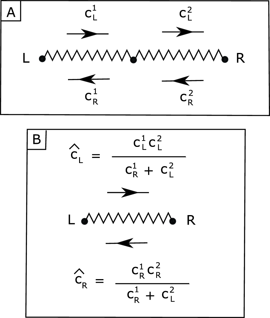
7.1.1 Components in SeriesFig. 1

Two electrical components in series connecting the nodes L and R (diagram A). The equivalent single electrical component with effective conductivities (diagram B)

Consider two electrical components connected in series with component 1 on the left of component 2 as in Fig. 1. The vertex set of the graph is here given by just three points; dropping the N subscript and labelling the intermediate node as M we have \(\Omega =\\) with boundary nodes \(\partial \Omega = \\). We denote by \(c^i_L\) (\(c^i_R\)) the left (right) conductivity of the \(i^\textrm\) component, and we suppose that \(c^1_R+ c^2_L>0\). From the random walk perspective, this latter condition is rather natural since when it is violated the walker is trapped in the middle point and consequently charge accumulates there (see also the similar discussion at the start of Sect. 5.4).

We now put the two extremes in contact with fixed potentials \(\lambda _L\) and \(\lambda _R\) at L and R, respectively. Trivially, any current with zero divergence on \(\\) satisfies \(j(L,M)=j\) and \(j(M,R)=j\) for some \(j\in \mathbb \). If the current j is fixed, then the optimum potential \(\phi _M\) at the junction point M between components 1 and 2 is obtained by minimizing the sum of the energies; using Lemma 5.2 we thus have

$$\begin \inf _\left[ }_^(j)+}_^(j)\right]&= \inf _\left[ \Gamma _(j)+\Gamma _(j)\right] \nonumber \\&=\Gamma _,\lambda _R\frac}(j) \nonumber \\&=}_^,\frac }(j)\,. \end$$

(7.3)

Let us next imagine that the above electrical components are part of a larger network, but still with an intermediate node M shared only by these two components in series. As long as the value of the potential \(\phi _M\) is not fixed and not relevant, then the node M can be removed and the two electrical components in series can be substituted by one single electrical component having effective left and right conductivities \(}_L\), \(}_R\) given, respectively, by

$$\begin }_L=\frac, \qquad }_R= \frac. \end$$

(7.4)

Note that the above expressions are not symmetric under the exchange of 1 and 2, but we recover the classic rules of electrical networks when \(c^i_L=c^i_R\).

7.1.2 Components in Parallel

Turning now to investigate electrical components in parallel, we begin with a simple observation:

Lemma 7.1

For each \( j \in \mathbb \) we have

$$\begin \inf _}\big \(j_1)+\Gamma _(j_2)\}= \Gamma _(j) . \end$$

(7.5)

Proof Fig. 2

Two electrical components in parallel connecting the nodes L and R (diagram A). The equivalent single electrical component with effective conductivities (diagram B)

The proof of this lemma can be obtained simply by a probabilistic argument. Let \(N^_T\), \(N^_T\), \(N^_T\), \(N^_T\) be independent Poisson processes. The joint rate functional for the pair \(\frac\left( N^_T-N^_T,N^_T-N^_T\right) \) is given by \((j_1,j_2)\mapsto \Gamma _(j_1)+\Gamma _(j_2)\). By the contraction principle, the rate functional for the sum of the two components of the pair is then given by the left-hand side of (7.5). However, we also have that the sum of the components has the same distribution as \(\frac\left( N^_T-N^_T\right) \), whose rate functional is the right-hand side of (7.5). \(\square \)

The above lemma implies the following rule of equivalence for two electrical components connected in parallel. Consider again component 1 with left (right) conductivity \(c^1_L\) (\(c^1_R\)) and component 2 with left (right) conductivity \(c^2_L\) (\(c^2_R\)). We now arrange the two components so that their left and right extremes are coincident and set to potentials \(\lambda _L\) and \(\lambda _R\), respectively (see Fig. 2). The cost when current \(j_1\) crosses component 1 and current \(j_2\) crosses component 2 is given by

$$\begin }_^(j_1)+ }_^(j_2). \end$$

(7.6)

When the potentials \(\lambda _L\), \(\lambda _R\) are fixed, and we are not interested in the exact currents flowing across each of the two components, but only in the total current flowing between the two nodes, then the cost associated to a total current j is obtained minimizing (7.6) under the constraint \(j_1+j_2=j\). Indeed, by Lemma 7.1, the minimum of (7.6) over all \(j_1\) and \(j_2\) such that \(j_1+j_2=j\) is given by \(}_^(j)\). This means that the pair of electrical components can be substituted by one single component having effective conductivities given by

$$\begin }_L=c^1_L+c^2_L, \qquad }_R=c^1_R+c^2_R. \end$$

(7.7)

7.1.3 Star-Triangle Relation

The star-triangle transformation allows us to replace a star graph with three rays by a triangle as in Fig. 3. While in the classic theory of electrical networks there are transformations in both directions, here we will have a transformation from the star to the triangle but generally not the reverse. Note that going from the star to the triangle decreases by one the number of vertices and thus reduces the complexity of the network. We label the vertices of the star A, B, C and O; only the boundary nodes A, B and C are retained in the triangle.

To be concrete, the equivalence holds and we can replace the star by the triangle as long as we do not observe the potential in the central node O of the star and simply impose that the total current entering/exiting from each node of the triangle through the edges of the triangle is identical to that in the star with the same potentials on the boundary nodes (see Lemma 7.2 for a precise statement).

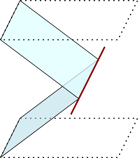
Fig. 3

Geometry of the star-triangle relation. Non-reversible components on the links of the star at the top are to be replaced by effective components on the links of the triangle at the bottom Maybe it would be nice, if possible, to have this and the other figures aligned orizontally

We denote the hopping rates (conductivities) in the star by c(A, O), c(B, O), c(C, O), c(O, A), c(O, B), c(O, C) and those in the triangle by \(\widehat(A,B)\), \(\widehat(B,C)\), \(\widehat(C,A)\), \(\widehat(B,A)\), \(\widehat(C,B)\), \(\widehat(A,C)\). The algebraic relations between conductivities which have to be satisfied in order that a star-triangle relation may hold are not that easily guessed, but some clues come from considering the special cases when one among j(A, O), j(B, O) and j(C, O) is identically zero. It turns out that when the conductivities c are fixed, the conductivities \(}\) are uniquely determined by

$$\begin \left\ \widehat(A,B)=\frac,\\ \widehat(B,A)=\frac,\\ \widehat(B,C)=\frac,\\ \widehat(C,B)=\frac,\\ \widehat(C,A)=\frac,\\ \widehat(A,C)=\frac.\\ \end \right. \end$$

(7.8)

Further intuition and a formal justification of these transformations are given later in this section with a natural interpretation in terms of the trace process in Sect. 7.3.

We first discuss the inversion of (7.8). To show that this is not possible in general we observe that, if we construct the product of the conductivities \(}\) obtained in the previous formulas, we obtain the same result going clockwise or anticlockwise in the triangle, i.e. we have

$$\begin \widehat(A,B)\widehat(B,C)\widehat(C,A)=\widehat(A,C)\widehat(C,B)\widehat(B,A). \end$$

(7.9)

The reverse procedure is therefore possible only when (7.9) is satisfied. Moreover, even in this case, the conductivities c are not uniquely defined as we now show.

We first state two simple facts that will be useful in the following. Consider the system of equations in the variables x, y, z given by

$$\begin \left\ x=a_1y\\ y=a_2z\\ z=a_3x \end \right. \end$$

(7.10)

where \(a_1\), \(a_2\), \(a_3\) are real numbers such that \(a_1a_2a_3=1\). Equations (7.10) have a one-parameter family of solutions given by

$$\begin x=\left( \frac\right) ^}\ell ,\ \ \ y=\left( \frac\right) ^}\ell ,\ \ \ z=\left( \frac\right) ^}\ell , \ \ \ \ell \in }. \end$$

(7.11)

Consider also the system of equations in the variables x, y, z given by

$$\begin \left\ b_1=\frac\\ b_2=\frac\\ b_3=\frac\\ \end \right. \end$$

(7.12)

with \(b_1\), \(b_2\), \(b_3\) real numbers. Equations (7.12) have a unique solution given by

$$\begin x=\frac, \ \ y=\frac, \ \ z=\frac. \nonumber \\ \end$$

(7.13)

Using these facts we now consider inverting (7.8). Let us introduce the notation \(}(X,Y):=\frac}(X,Y)}}(Y,X)}\) where X and Y are any two of A, B and C. Likewise we define \((X,O):=\frac\) where X is A, B or C. Using (7.8), we obtain the equations

$$\begin \left\ (A,O)=}(A,B)(B,O)\\ (B,O)=}(B,C)(C,O)\\ (C,O)=}(C,A)(A,O)\\ \end \right. \end$$

(7.14)

which, since \(}(A,B)}(B,C)}(C,A)=1\) due to (7.9), have a one-parameter family of solutions

$$\begin & (A,O)=\left( \frac}(A,B)}}(C,A)}\right) ^}\ell ,\ \ \ (B,O)=\left( \frac}(B,C)}}(A,B)}\right) ^}\ell ,\ \nonumber \\ & (C,O)=\left( \frac}(C,A)}}(B,C)}\right) ^}\ell , \end$$

(7.15)

where \(\ell \in }^+\) as in (7.11). From (7.8) we can also get equations relating the three variables c(O, A), c(O, B), c(C, O) to \((A,O)\), \((B,O)\), \((C,O)\):

$$\begin \left\ \frac(A,B)}(A,O)}=\frac\\ \frac(B,C)}(B,O)}=\frac\\ \frac(C,A)}(C,O)}=\frac. \end \right. \end$$

(7.16)

By (7.13) the solution to the above system of equations is

$$\begin \left\ c(O,A)=\frac\frac(A,B)\widehat(B,C)}}(B,C)}}(C,A)}\right) ^}}+\frac(A,B)\widehat(C,A)}}(A,B)}}(B,C)}\right) ^}}+\frac(C,A)\widehat(B,C)}}(C,A)}}(A,B)}\right) ^}}}(B,C)}}(B,C)}}(A,B)}\right) ^}}}\\ c(O,B)=\frac\frac(A,B)\widehat(B,C)}}(B,C)}}(C,A)}\right) ^}}+\frac(A,B)\widehat(C,A)}}(A,B)}}(B,C)}\right) ^}}+\frac(C,A)\widehat(B,C)}}(C,A)}}(A,B)}\right) ^}}}(C,A)}}(C,A)}}(B,C)}\right) ^}}}\\ c(O,C)=\frac\frac(A,B)\widehat(B,C)}}(B,C)}}(C,A)}\right) ^}}+\frac(A,B)\widehat(C,A)}}(A,B)}}(B,C)}\right) ^}}+\frac(C,A)\widehat(B,C)}}(C,A)}}(A,B)}\right) ^}}}(A,B)}}(A,B)}}(C,A)}\right) ^}}}, \end \right. \end$$

(7.17)

and hence we see that the conductivities from the central node to the boundaries of the star are not uniquely defined but depend on the free parameter \(\ell \in }^+\). Finally, we can obtain the values \(c(A,O)=c(O,A)(A,O)\), \(c(B,O)=c(O,B)(B,O)\) \(c(C,O)=c(O,C)(C,O)\) and see, in contrast, that the conductivities from the boundaries to the central node are fixed numbers and do not depend on the free parameter \(\ell \).

Formally, the star-triangle transformation follows by the following statement.

Lemma 7.2

For any \(\phi _A,\phi _B,\phi _C\ge 0\) and for any j(A, O), j(B, O), j(C, O) such that \(j(A,O)+j(B,O)+j(C,O)=0\), we have

$$\begin \inf _&\left\(j(A,O)) +\Gamma _(j(B,O))\right. \nonumber \\ &\qquad \left. +~ \Gamma _(j(C,O))\right\} \nonumber \\&\quad = \inf \left\(A,B),\phi _B\widehat(B,A)}(j(A,B))+\Gamma _(B,C),\phi _C\widehat(C,B)}(j(B,C)) \right. \nonumber \\ &\qquad \left. +~\Gamma _(C,A),\phi _A\widehat(A,C)}(j(C,A))\right\} \end$$

(7.18)

where the \(\inf \) on the right-hand side is over

$$\begin&\left\ \end$$

(7.19)

and where the conductivities involved are related by (7.8) or equivalent formulation.

Proof

A proof by a direct computation is highly non-trivial; we present here a probabilistic proof. Since the rate functionals that we are interested in are the same for any superlinear zero-range process, we consider independent particles. We start from the star geometry and interpret it as a graph with one single node \(\Omega _N=\\) in contact with three ghost sites \(\partial \Omega _N=\\). By formula (4.1) the large deviation rate functional for the current through the edges of this star is finite only on currents that satisfy the zero-divergence condition at O, which is one of the hypotheses of the lemma; in that case the finite value of the rate functional is given by the left-hand side of (7.18).

We now do a higher-level large deviation principle; rather than just observing the flow across the edges of the star, we label particles and for each of them we look at the boundary site where it is created and the boundary site where it exits. By remark A.1 we can imagine that the particles that are created at O from the different boundaries immediately jump outside the system, since the large deviation rate functionals for long times are invariant with respect to how long particles spend on the site. Note that a particle at O will exit from site X, with \(X=A,B,C\) with probability, respectively, \(p_X:=\frac\). We can represent the dynamics of the particles using independent Poisson processes with a “thinning” construction as described in the following paragraphs.

Given a Poisson process \((N^\lambda _T)_}^+}\) of parameter \(\lambda \), we denote by \(}_(N_T^\lambda )\), (with \(0\le p_i\le 1\) and \(\sum _ip_i=1\)), the processes obtained by thinning of the process \(N^\lambda _T\); a point of \(N^\lambda _T\) belongs to \(}_(N^\lambda _T)\) with probability \(p_i\) independently from all the other points. The processes \(}_(N^\lambda _T)\) are independent Poisson processes of parameters \(p_i\lambda \).

Our construction is the following. The number of particles injected onto O from boundary site X (\(X=A,B,C\)) is given by the Poisson process \(N^_T\) and the three processes are independent. We perform an independent thinning procedure for each of them obtaining a family of independent Poisson processes \(\left( }_(N^)\right) _\). The process \(}_(N^)\) represents the number of particles created from the ghost site X and exiting through Y, and we can imagine that such particles go directly from X to Y through the edge (X, Y) of the triangle in the top of Fig. 3. The currents along the edges of the triangle are therefore given by

$$\begin j_T(X,Y)=\frac\left[ }_(N^)-}_(N^)\right] , \qquad X,Y=A,B,C, \nonumber \\ \end$$

(7.20)

and, since all the Poisson processes are independent, we have that the joint large deviation principle for these currents is given by

$$\begin&\Gamma _(A,B),\phi _B\widehat(B,A)}(j(A,B))+\Gamma _(B,C),\phi _C\widehat(C,B)}(j(B,C))\\ &\quad + \Gamma _(C,A),\phi _A\widehat(A,C)}(j(C,A)) \end$$

with the \(\widehat(X,Y)\) as in (7.8). Finally, the currents along the edges of the star are related to those on the edges of the triangle by (7.19) so the right-hand side of (7.18) is obtained by the contraction principle. The proof is finished. \(\square \)

7.2 Star-\(K_n\) Transformations

Lemma 7.2 can be generalized to a star with n non-central (boundary) nodes labelled \(X_1, X_2, \ldots X_n\) each linked to the same central node O. This n-ray star can be transformed to an equivalent n-complete graph where the central node is removed and each of the n boundary nodes is linked to each of the other \(n-1\) nodes. Using a similar argument to the previous subsection, the effective conductivity \(\widehat(X_i,X_j)\) going from boundary node \(X_i\) to boundary node \(X_j\) must be given in terms of conductivities in the star by

$$\begin \widehat(X_i, X_j)=\frac^N c(O,X_i)}. \end$$

7.3 Trace Process

Given X(t) the random walk on \((\Omega _N\cup \partial \Omega _N,E_N)\) with jump rates \((c(x,y))_\) and \(S\subset \Omega _N\cup \partial \Omega _N \); we can construct the corresponding trace process \(X^S(t)\) which is still a Markov process on \(((\Omega _N\cup \partial \Omega _N)\setminus S, E'_N)\) with \(E'\) a suitable set of edges. For the general construction and proofs we refer to [23]; here we consider just the case when S is a single node in \(\Omega _N\).

Given a node \(x\in \Omega _N\) the corresponding trace process \(X^x(t)\) is most naturally defined in terms of trajectories. Let \((X(t))_\) be a trajectory of the original random walk, and let \(I_i\subseteq [0,T]\) be the time intervals when the walker is at \(\\). The trajectory \(\left( X^x(t)\right) _\) of the trace process is obtained cutting out all the periods that the walker spends at x and gluing back together the pieces of trajectories obtained. The process obtained in this way is still Markov, and in the case of deletion of one single node the new transition graph and the new rates are exactly the ones obtained by the star-\(K_n\) transformations; see [23] for proofs and more details. This also leads to a relation of our construction with harmonic functions which we will not discuss further here.