
Remember me


99mTc-TRODAT-1 SPECT data of 100 patients with suspected PD (age range: 35 to 87 years, mean ± standard deviation (SD): 70.88 ± 9.84 years; injected activity: 1110 MBq; 55 male and 45 female) were retrospectively collected in 2016 from Show Chwan Memorial Hospital under the local ethics approval (SCMH_IRB Number, 1311110704). All data were acquired using a commercial clinical dual-head SPECT/CT scanner (Symbia, Siemens Healthineers, Erlangen, Germany) equipped with 2 low-energy high-resolution parallel-hole collimators, and a 9.6 mm (3/8 inch) thick NaI crystal with a 3.8 mm intrinsic resolution. The dual energy window (DEW) scatter correction method was implemented, with the primary and scatter windows set at 126–154 keV and 114–126 keV, respectively. The SPECT data comprised of 120 projection views with a bin size of 2.7 mm. CT images were acquired for SPECT AC after the SPECT scan using a 2-slice CT scanner with acquisition parameters of 10 mAs, 130 kVp, a pitch of 1.5, and a reconstructed slice thickness of 3 mm. The CT images were subsequently registered to SPECT data using the scanner software and then converted to µ-maps using a bilinear model [27].
Simulation datasetWe generated a population of 200 realistic digital PD phantoms based on our previous study [28]. The MC simulation tool SIMIND [19] was used to generate realistic simulated projection data modeling all relevant physical factors as well as the same SPECT system and data acquisition parameters as the clinical data. Almost noise-free projections with 120 views and a 1 mm bin size were obtained by about 50 M simulated photon counts. Projections were then resampled from 256 × 200 × 120 to 95 × 74 × 120 with a 2.7 mm bin size consistent with clinical data to model continuous-to-discrete activity sampling in clinical data acquisition [29]. We also generated a set of analytical simulation projections, modeling only the attenuation effect using a rotation based analytical projector [30]. We then scaled both MC and analytical simulation projections following a truncated Gaussian distribution according to our clinical reference (2.49 ± 0.73 M, range 0.49 ~ 4.88 M), and modeled Poisson noise on the scaled projections to obtain realistic noisy simulated projections.
The reconstruction process utilized ordered subset expectation maximization algorithm (8 iterations, 4 subsets). Both clinical and simulation projections were reconstructed with and without CT-based AC (CTAC and NAC). Additionally, ChangAC for clinical data was implemented for comparison. DEW scatter correction and collimator-detector response correction were applied for both clinical and MC simulated data. The reconstructed images were with a matrix size of 128 × 128 × 128 and a voxel size of 2.7 × 2.7 × 2.7 mm³. A Gaussian filter with a full-width-at-half-maximum of 4.8 mm was applied to all reconstructed images. Sample images of simulated and clinical CTAC data were presented in Supplementary Fig. 1.
Network architectureIn this study, a 3D cGAN was implemented [14], consisting of a U-Net generator (G) and a convolutional neural network (CNN) discriminator (D). The U-Net generator consisted of four encoder-decoder layers, each included two convolutional layers with a kernel size of 3 × 3 × 3, followed by a rectified linear unit (ReLU) activation function. After the activation function, a 3D max-pooling layer with a stride of 2 and a kernel size of 2 × 2 × 2 was used for each encoding step, and transposed convolutional layers were used to recover the feature maps for the decoding step. The recovered feature maps were concatenated with the skip connection from the corresponding encoder layer and served as input for the subsequent decoder layer. After the final decoder layer, a convolutional layer with a kernel size of 1 × 1 × 1 was employed to produce the final estimated data as the network output.
The discriminator consisted of four 3D convolutional layers with a stride of 2 and a kernel size of 3 × 3 × 3. Each convolutional layer was followed by a leaky ReLU (LReLU) activation function with a slope of 0.2. CTAC images and DL-based AC images from the generator were used as input. Then a binary classification was made to evaluate the authenticity of the input images. The generator loss \(\:_\) and the discriminator \(\:_\) were defined as follows:
$$\:\begin_\left(x,y\right)=_\left(x\right)+\lambda\:_(G\left(x\right),y)\end$$
(1)
$$\:\begin_\left(x,y\right)=\frac\left(\right(D\left(x,y\right)-_^+\left(D\right(x,G\left(x\right)-_^)\end$$
(2)
Where \(\:x\) and \(\:y\) were the NAC and CTAC SPECT image, respectively. \(\:_\) was the adversarial loss function of the generator, \(\:_\) was the smooth \(\:_\) loss function, which combines the advantages of \(\:_\) and \(\:_\) loss. They were defined as follows:
$$\:\begin_\left(x\right)=\frac\left(\right(D\left(x\right),G\left(x\right)-_^\end$$
(3)
$$\:\begin_\left(x,y\right)=\left\\frac(y-G\left(x\right)^,\:\:\:\left|y-G\left(x\right)\right|<1\\\:\left|y-G\left(x\right)\right|-0.5,\:\:\:\:\:\:otherwise\end\right.\end$$
(4)
where \(\:_\)=1 and \(\:_\)=0 were labels for the discriminant results of real and synthetic images, respectively. λ was the weight for \(\:_\) loss and is set to 10 in this study [31]. The proposed network was trained for 600 epochs with an initial learning rate of 0.0002, employing the Adam optimizer for optimization [32]. The network was implemented using PyTorch and executed on a NVIDIA GeForce RTX 4090 GPU.
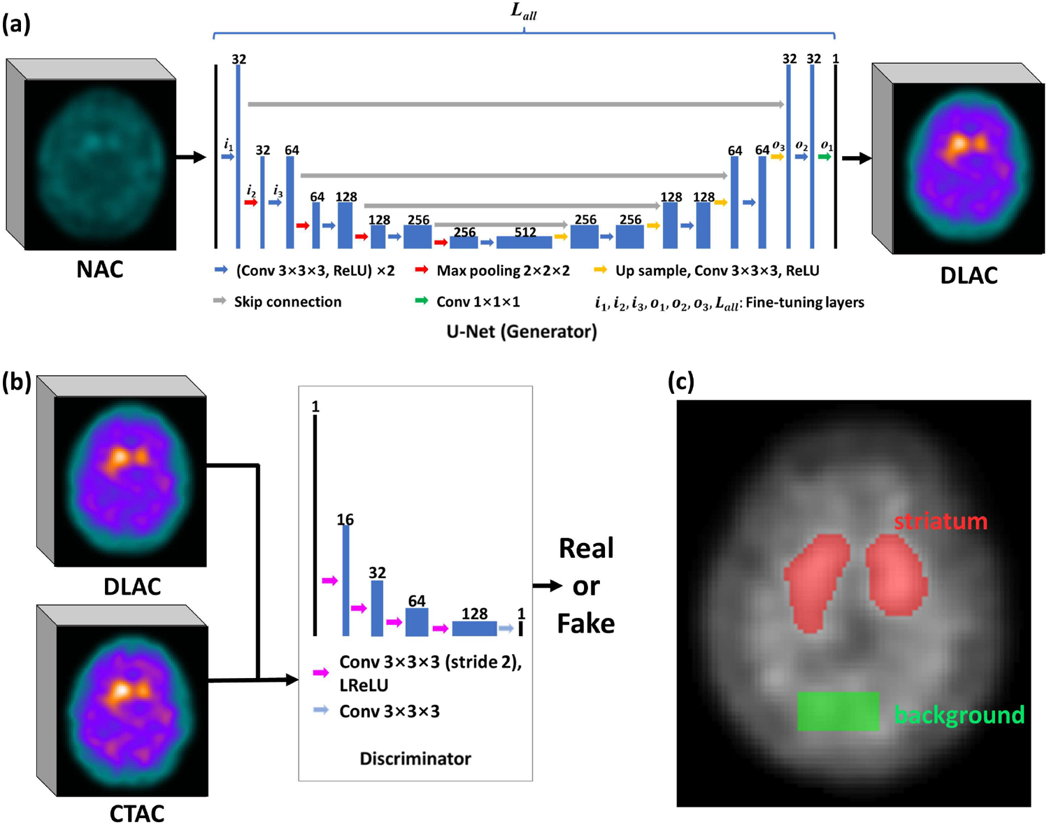
Fig. 1
The schematic diagram of the 3D cGAN architecture used in this study. (a) The U-Net generator and (b) the discriminator. The layers for fine-tuning are labeled on the U-Net generator. (c) Striatum (red mask) and background (green mask) regions-of-interest used in this study
Network trainingThe 3D cGAN was first pre-trained by 200 paired MC or analytical simulated NAC and CTAC DAT SPECT images to get the pre-trained model, respectively. Subsequently, 8, 24, and 80 pairs of NAC and CTAC clinical DAT SPECT images were employed to fine-tune the pre-trained MC simulation model (TLAC-MC) and analytical simulation model (TLAC-ANA). The FT process for TLAC-MC involved 3 different strategies: (i) TLAC-MC-st1: FT the first input layer i1 and the last output layer o1; (ii) TLAC-MC-st2: FT the first three down-sampling layers (\(\:_,_,_\)) and the last three up-sampling layers (\(\:_,_,_\)); (iii) TLAC-MC-st3: FT all layers (n = 18) \(\:_\). Best FT strategy would be was used for TLAC-MC and TLAC-ANA later in the study for further comparison. The FT layers were depicted in Fig. 1a. Given the same number of available clinical data used for FT in TLAC, i.e., 8/24/80, various training strategies were also implemented for comparison, including training using limited amount (8/24/80) of clinical data (DLAC-CLI) as the baseline; with 6 times data augmentation (8 × 6/24 × 6/80 × 6) using ± 10 degrees rotations and horizontal flip of the clinical data (DLAC-AUG); with a direct mixture (8/24/80 clinical + 200 MC simulation) of data (DLAC-MIX); and direct testing using the pre-trained MC model without FT (DLAC-MC). All training datasets were split into 7/8 for training and 1/8 validation. For testing, 20 clinical data were tested for models trained on 80 clinical datasets, while 50 clinical data were tested for models trained on 24 or 8 clinical datasets. All 100 clinical data were tested for DLAC-MC as a single fold. A 5-fold cross-validation was applied to training strategies utilizing 80 clinical datasets, while a 2-fold cross-validation was implemented for training strategies employing 24 or 8 clinical datasets to test all 100 clinical cases.
Evaluation metricsMC simulated CTAC images were compared with the clinical CTAC images using a voxel-based analysis of normalized mean square error (NMSE) (Eq. 5) and structural similarity index (SSIM) (Eq. 6) on the whole 3D brain region. Both indices were also assessed on clinical NAC, ChangAC, different DL-based AC images.
$$\:\beginNMSE=\frac^(_-_^}^_}^}\end$$
(5)
$$\:\begin\:\:\:\:\:\:\:SSIM=\frac__+_\right)\left(2_+_\right)}_^+_^_\right)\left(_^+_^_\right)}\end$$
(6)
where \(\:N\) was the total number of voxels, \(\:\lambda\:\) as the voxel count value in the reference image, i.e., clinical CTAC image, \(\:_\) was the voxel count value in evaluated image, and \(\:j\) was the voxel index. \(\:_\:\)and \(\:_\) were the mean value and standard deviation of the reference image, \(\:_\) and \(\:_\) were the mean value and standard deviation of the evaluated image,\(\:_\) was the cross-covariance between the evaluated image and the reference image. The constants \(\:_=_\times\:L^\) and \(\:_=_\times\:L^\) are used to stabilize the division when the denominator is very small. \(\:L\) represents the maximum voxel value between the 2 compared images. \(\:_\) and \(\:_\) are empirically set to 0.01 and 0.03 [33], respectively. Scatter plots of NMSE and SSIM results between reconstructed MC simulation and clinical data, as well as among clinical data were generated to evaluate the similarity between the two. A paired Mann-Whitney U test was used to evaluate their NMSE and SSIM differences, and was also employed to compare NMSE and SSIM results for different AC methods compared to their corresponding baseline method. For DL-based AC methods trained on different number of clinical datasets, their baselines were the DLAC-CLI models trained on the same number of clinical datasets. Meanwhile, NAC, ChangAC, and DLAC-MC were compared with DLAC-CLI trained on 8 clinical datasets. A p-value of < 0.05 indicates a significant difference. Joint histogram analysis and linear regression were also performed to evaluate the distribution differences between various AC methods and their corresponding baselines.
For clinically relevant analysis, striatal binding ratio (SBR) (Eq. 3) was assessed for different AC images.
$$\:\beginSBR=\frac}_-}_}}_}\end$$
(7)
where \(\:}_\) was the mean count value in the striatum region and \(\:}_\) was the mean count value in a uniform cerebellum region (20 × 10 × 10) (Fig. 1c). The striatum region was segmented using a threshold of 67% of the maximum intensity of the DAT SPECT images for each subject [34]. Bland-Altman plots were applied to SBR results to evaluate the differences among various AC methods compared to their corresponding baselines.
Comments (0)