The cost-effectiveness analysis was conducted using a hybrid model composed of a decision tree that captures short-term outcomes followed by a Markov model programmed in Excel, with a 10-year time horizon, to capture long-term outcomes. The structure of the model aims to capture the long-term treatment of a chronic condition such as AD. The design and implementation of the model was significantly informed by published literature [22] and other publicly available documentation reviewing and critiquing recent pharmacoeconomic modeling of treatments for AD [23, 24].

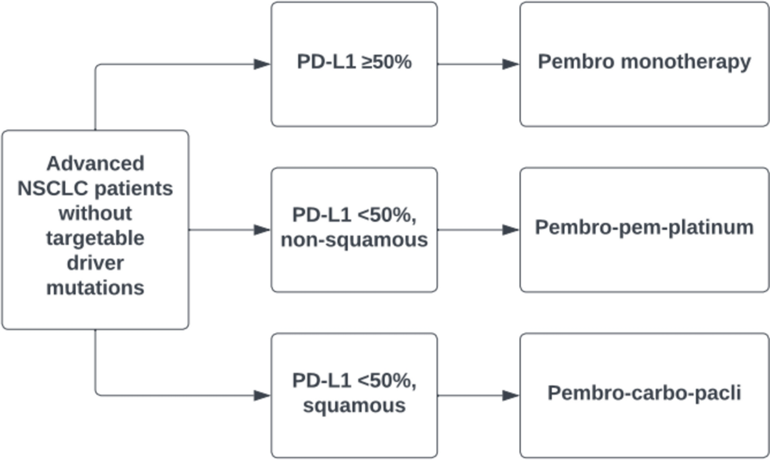
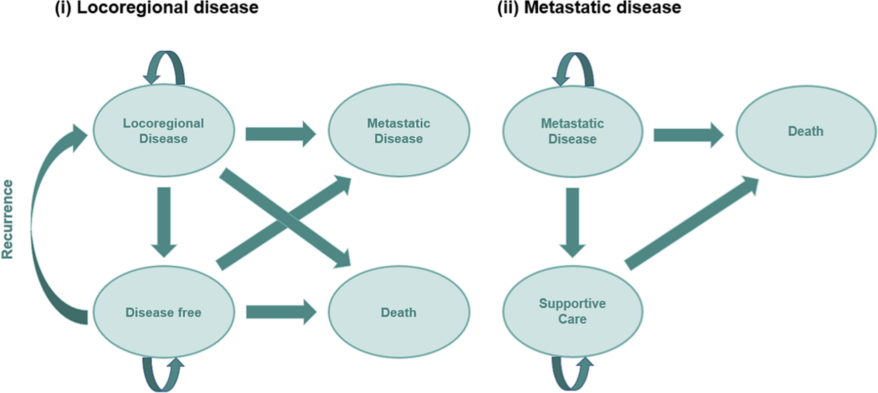
The model evaluated the costs and outcomes of adults with severe AD inadequately controlled with topical therapy or for whom topical therapies were medically inadvisable or required systemic treatment to control the disease. Patients entered the model through the decision tree (Fig. 1a), where they received abrocitinib or one of the comparators in combination with topical drug therapy. Response to treatment was assessed at 16 weeks as most of the included trials assessed their primary efficacy endpoint in this time period. Treatment response was defined by a ≥ 75% reduction in EASI score (EASI-75) after a patient began treatment. If patients responded to treatment and did not discontinue, they continued receiving the same intervention until week 52, when the response was again evaluated. If patients did not respond to treatment at any node of the decision tree, they were considered to stop treatment and start subsequent therapy.

Abrocitinib cost-effectiveness model structure. a Decision tree (until week 52); b Markov model (52+ weeks). AD atopic dermatitis

After 52 weeks, patients entered the Markov model (Fig. 1b) for long-term maintenance treatment, which consisted of three health states: maintenance with active therapy (abrocitinib or a comparator), subsequent treatment (in case of discontinuation or loss of response), or death. The simulation was conducted on a 6-month cycle length (with half-cycle correction) for the remainder of the time horizon. Patients who were still administered abrocitinib or a comparator following the first 52 weeks of treatment were treated continuously with that product until loss of response or treatment discontinuation (response was re-assessed after each cycle). When this occurred, patients transitioned to subsequent treatment, where they remained until death. Transition to death state (absorbing state) was possible from any health state.

The modelled population had a mean age of 34 years at the start of the model, based on the mean age of participants in abrocitinib studies [25]. The model considered age-dependent mortality data for the Spanish population obtained from the National Institute of Statistics mortality tables [27]. The presence of AD did not increase the likelihood of death.

All data inputs were validated by a panel including three Spanish clinical experts (two dermatologists and one hospital pharmacist) through an advisory board and follow-up one-to-one consultations [28].

Key efficacy inputs used in the model included the time to onset of response, the response at 16 and 52 weeks (decision tree), the annual loss of treatment response (Markov model), and the discontinuation both in the year of treatment initiation and each year after that (decision tree and Markov model).

As described above, the response was defined as EASI-75 score (Table 1). The model assumed patients in treatment with JAK inhibitors begin experiencing therapeutic benefits at 8 weeks, as supported by clinical trial results that suggest response to abrocitinib commonly emerges within 4 weeks and has typically plateaued by 8 weeks [29]. For injectable medications (dupilumab and tralokinumab), it was assumed responders begin experiencing benefits at 16 weeks, as supported by clinical studies [29, 30].

Response rates are detailed in Table 1. The percentage of responders at 16 weeks was derived from a network meta-analysis for abrocitinib 200 mg, dupilumab 300 mg, tralokinumab 300 mg, and baricitinib 2 and 4 mg [31]. For upadacitinib 15 and 30 mg, response rates were derived from the AD-Up study [19].

Loss of treatment response beyond 52 weeks was assumed to occur at the same rate observed between 16–52 weeks (derived with reference to the proportion of week 16 responders who sustained response at week 52 based on the clinical trials of each comparator).

Due to the lack of treatment discontinuation rates for each treatment, it was assumed to be the same for all comparators: 6.9% of patients discontinued during the first 52 weeks (based on rates observed for EASI-75 responders discontinuing abrocitinib 200 mg in JADE EXTEND) [32], and 6.3% discontinued each subsequent year (based on results from LIBERTY AD SOLO for dupilumab) [23].

The analysis applied health state utilities based on EuroQol instrument (EQ-5D-3L) data collected in two dupilumab phase III clinical trials for adults with moderate-to-severe AD [33] (Table 1), in line with NICE recommendations [24]. EQ-5D-3L is a standardized health-related quality of life (HRQoL) questionnaire which evaluates five dimensions (mobility, self-care, usual activities, pain/discomfort, and anxiety/depression) in three levels of severity. Utilities reported range from 0 (death) to 1 (perfect health).

In addition, the model applied adjustment factors that accounted for the HRQoL impact of Spanish cohort aging [34]. Population norms were applied multiplicatively to treatment state utilities to reflect the aging of the cohort beyond its average age upon initiation of treatment and the resultant decline in baseline utility over time.

Costs included drug-related costs (acquisition and administration), adverse events (AEs) management, testing, medical visits and hospitalizations, and cost of subsequent treatment. All costs were presented in 2022 euros (€).

Drug costs were calculated using list prices obtained from the database of the Official College of Pharmacists [37] (the rebate established in Spanish Royal Decree-Law 8/2010 was applied [37]). In addition, a one-time cost of training patients to self-administer injectable products (specialized nursing visit) was included for dupilumab and tralokinumab (Table 2). No administration costs were considered for oral therapies.

Annual testing was assumed to be the same for all comparators. For AE management, the model included those experienced by at least 5% of participants in clinical trials for any comparator [29, 38,39,40,41]. Frequencies of AEs were annualized (Table S1, see electronic supplementary material [ESM]). AEs were assumed to be usually managed through a visit to a dermatologist or an ophthalmologist for allergic conjunctivitis (Table 2).

The model also accounted for the costs of primary care visits, emergency room visits, and hospitalizations depending on treatment response. The average annual utilization of each resource was derived from a longitudinal, non-interventional, retrospective cohort study in Canadian patients with AD [42], and Spanish unitary costs [43] were applied (Table 2).

For subsequent treatment, experts assumed an average cost between biological drugs and JAK inhibitors, considering the highest price of each category, in order not to underestimate the cost of this state (Table 2).

The model reported outputs including total costs, years in response, years in subsequent therapy and quality-adjusted life-years (QALYs). The incremental cost per QALY gained was calculated. A willingness-to-pay (WTP) threshold of €25,000 per QALY gained was considered in line with the Spanish guidelines [44]. If the incremental cost-effectiveness ratio (ICER) of the treatment was below the WTP threshold, then it was considered a cost-effective alternative. When the intervention was both clinically superior and cost saving, it was referred to as an economically ‘dominant’ strategy. The opposite was a ‘dominated’ strategy. Another option is that an alternative was less costly, but also less effective.

Both costs and outcomes were discounted at 3% per year according to the local recommendations for economic evaluation of health technologies [45, 46].

One-way sensitivity analysis (OWSA), scenario and probabilistic sensitivity analyses (PSA) were carried out to identify the most influential parameters and test the robustness of the results.

OWSA was performed to investigate the impact of individual model parameters used in the base-case analysis on model outcomes, using the hypothetical increases or decreases of 20%. Finally, results were compared with the base case in a tornado diagram.

The PSA was conducted using a Montecarlo simulation with 1000 iterations. A PSA simultaneously sets all inputs to a value randomly sampled from the appropriate distribution (Table S2, see ESM). When uncertainty data were not reported, the standard error was assumed to be 10% of the mean.

A scenario analysis was performed for a 5-year time horizon. To further account for the structural uncertainty, alternative scenarios were constructed to assess the impact of variations in discontinuation rates on cost effectiveness (i.e. maintaining the values of abrocitinib for 16–52 weeks and dupilumab for +52 weeks and increasing the other values by 10% [scenario 1] or decreasing the other values by 2% [scenario 2]; using the same values for the same drug type, and increasing or decreasing the others by 2% [scenario 3 and 4]; Table S3, see ESM).

The NNT is an outcome measure commonly used in clinical settings, providing a quick, short-hand approach to estimating relative efficacy of different treatments [47]. The NNT corresponds to the average number of patients who need to be treated with a particular therapy to achieve one extra positive outcome when compared with another therapy or placebo. The ideal NNT is 1 because it implies every patient treated will achieve the stated clinical benefit. The higher the NNT, the less effective the intervention [48].

NNT is often used as a tool in medical decision-making [47]. For this reason, we additionally included an analysis of the cost per NNT for abrocitinib 200 mg and dupilumab 300 mg based on EASI-75 responders from a post-hoc analysis of patients with severe AD from the JADE COMPARE study [21, 49], as these are the unique treatments that have been compared in a head-to-head study. Firstly, the NNT for achieving an EASI-75 response was obtained using the difference in response for active treatment (abrocitinib 200 mg or dupilumab 300 mg) versus placebo at 12 and 16 weeks, where the NNT is calculated as the inverse of the probability of response to the active treatment minus the probability of response to placebo.

The cost per NNT for each drug was obtained by multiplying the annual cost of each therapy over the first year of treatment by its NNT (at 12 and 16 weeks).

Additionally, NNT for abrocitinib versus dupilumab was calculated. An incremental cost per additional patient with clinically meaningful outcome was calculated as the difference in annual drug costs (abrocitinib vs dupilumab) multiplied by the corresponding NNT. When the difference in total cost is negative and the NNT is positive, the incremental cost per additional patient is denoted as ‘dominant’.